Simple-effect analysis and post-hoc multiple comparison.

Perform (1) simple-effect (and simple-simple-effect) analyses, including both simple main effects and simple interaction effects, and (2) post-hoc multiple comparisons (e.g., pairwise, sequential, polynomial), with p values adjusted for factors with >= 3 levels.

This function is based on and extends (1) emmeans::joint_tests(), (2) emmeans::emmeans(), and (3) emmeans::contrast(). You only need to specify the model object, to-be-tested effect(s), and moderator(s). Almost all results you need will be displayed together, including effect sizes (partial \(\eta^2\) and Cohen's d) and their confidence intervals (CIs). 90% CIs for partial \(\eta^2\) and 95% CIs for Cohen's d are reported.

By default, the root mean square error (RMSE) is used to compute the pooled SD for Cohen's d. Specifically, it uses:

the square root of mean square error (MSE) for between-subjects designs;
the square root of mean variance of all paired differences of the residuals of repeated measures for within-subjects and mixed designs.

Disclaimer: There is substantial disagreement on the appropriate pooled SD to use in computing the effect size. For alternative methods, see emmeans::eff_size() and effectsize::t_to_d(). Users should not take the default output as the only right results and are completely responsible for specifying sd.pooled.

Usage

EMMEANS(
  model,
  effect = NULL,
  by = NULL,
  contrast = "pairwise",
  reverse = TRUE,
  p.adjust = "bonferroni",
  sd.pooled = NULL,
  model.type = "multivariate",
  digits = 3
)

Arguments

model

The model object returned by MANOVA.

effect

Effect(s) you want to test. If set to a character string (e.g., "A"), it reports the results of omnibus test or simple main effect. If set to a character vector (e.g., c("A", "B")), it also reports the results of simple interaction effect.

by

Moderator variable(s). Defaults to NULL.

contrast

Contrast method for multiple comparisons. Defaults to "pairwise".

Alternatives can be "pairwise" ("revpairwise"), "seq" ("consec"), "poly", "eff". For details, see ?emmeans::`contrast-methods`.

reverse

The order of levels to be contrasted. Defaults to TRUE (higher level vs. lower level).

p.adjust

Adjustment method of p values for multiple comparisons. Defaults to "bonferroni". For polynomial contrasts, defaults to "none".

Alternatives can be "none", "fdr", "hochberg", "hommel", "holm", "tukey", "mvt", "dunnettx", "sidak", "scheffe", "bonferroni". For details, see stats::p.adjust() and emmeans::summary().

sd.pooled

By default, it uses sqrt(MSE) (root mean square error, RMSE) as the pooled SD to compute Cohen's d. Users may specify this argument as the SD of a reference group, or use effectsize::sd_pooled() to obtain a pooled SD. For an issue about the computation method of Cohen's d, see Disclaimer above.

model.type

"multivariate" returns the results of pairwise comparisons identical to SPSS, which uses the lm (rather than aov) object of the model for emmeans::joint_tests() and emmeans::emmeans().

"univariate" requires also specifying aov.include=TRUE in MANOVA (not recommended by the afex package; for details, see afex::aov_ez()).

digits

Number of decimal places of output. Defaults to 3.

Value

The same model object as returned by MANOVA (for recursive use), along with a list of tables: sim (simple effects), emm (estimated marginal means), con (contrasts).

Each EMMEANS(...) appends one list to the returned object.

Interaction Plot (See Examples Below)

You can save the returned object and use the emmeans::emmip() function to create an interaction plot (based on the fitted model and a formula). See examples below for the usage.

Note: emmeans::emmip() returns a ggplot object, which can be modified and saved with ggplot2 syntax.

Statistical Details

Some may confuse the statistical terms "simple effects", "post-hoc tests", and "multiple comparisons". Such a confusion is not uncommon. Here I explain what these terms actually refer to.

1. Simple Effect

When we speak of "simple effect", we are referring to ...

simple main effect
simple interaction effect (only for designs with 3 or more factors)
simple simple effect (only for designs with 3 or more factors)

When the interaction effect in ANOVA is significant, we should then perform a "simple-effect analysis". In regression, we call this "simple-slope analysis". They are identical in statistical principles.

In a two-factors design, we only test "simple main effect". That is, at different levels of a factor "B", the main effects of "A" would be different. However, in a three-factors (or more) design, we may also test "simple interaction effect" and "simple simple effect". That is, at different combinations of levels of factors "B" and "C", the main effects of "A" would be different.

To note, simple effects per se never require p-value adjustment, because what we test in simple-effect analyses are still "omnibus F-tests".

2. Post-Hoc Test

The term "post-hoc" means that the tests are performed after ANOVA. Given this, some may (wrongly) regard simple-effect analyses also as a kind of post-hoc tests. However, these two terms should be distinguished. In many situations, "post-hoc tests" only refer to "post-hoc comparisons" using t-tests and some p-value adjustment techniques. We need post-hoc comparisons only when there are factors with 3 or more levels.

Post-hoc tests are totally independent of whether there is a significant interaction effect. It only deals with factors with multiple levels. In most cases, we use pairwise comparisons to do post-hoc tests. See the next part for details.

3. Multiple Comparison

As mentioned above, multiple comparisons are indeed post-hoc tests but have no relationship with simple-effect analyses. Post-hoc multiple comparisons are independent of interaction effects and simple effects. Furthermore, if a simple main effect contains 3 or more levels, we also need to do multiple comparisons within the simple-effect analysis. In this situation, we also need p-value adjustment with methods such as Bonferroni, Tukey's HSD (honest significant difference), FDR (false discovery rate), and so forth.

Options for multiple comparison:

"pairwise" - Pairwise comparisons (default is "higher level - lower level")
"seq" or "consec" - Consecutive (sequential) comparisons
"poly" - Polynomial contrasts (linear, quadratic, cubic, quartic, ...)
"eff" - Effect contrasts (vs. the grand mean)

Examples

#### Between-Subjects Design ####
# \donttest{
between.1
#>    A SCORE
#> 1  1     3
#> 2  1     6
#> 3  1     4
#> 4  1     3
#> 5  1     5
#> 6  1     7
#> 7  1     5
#> 8  1     2
#> 9  2     4
#> 10 2     6
#> 11 2     4
#> 12 2     2
#> 13 2     4
#> 14 2     5
#> 15 2     3
#> 16 2     3
#> 17 3     8
#> 18 3     9
#> 19 3     8
#> 20 3     7
#> 21 3     5
#> 22 3     6
#> 23 3     7
#> 24 3     6
#> 25 4     9
#> 26 4     8
#> 27 4     8
#> 28 4     7
#> 29 4    12
#> 30 4    13
#> 31 4    12
#> 32 4    11
MANOVA(between.1, dv="SCORE", between="A") %>%
  EMMEANS("A")
#> 
#> ====== ANOVA (Between-Subjects Design) ======
#> 
#> Descriptives:
#> ─────────────────────
#>  "A"   Mean    S.D. n
#> ─────────────────────
#>   A1  4.375 (1.685) 8
#>   A2  3.875 (1.246) 8
#>   A3  7.000 (1.309) 8
#>   A4 10.000 (2.268) 8
#> ─────────────────────
#> Total sample size: N = 32
#> 
#> ANOVA Table:
#> Dependent variable(s):      SCORE
#> Between-subjects factor(s): A
#> Within-subjects factor(s):  –
#> Covariate(s):               –
#> ─────────────────────────────────────────────────────────────────
#>        MS   MSE df1 df2      F     p     η²p [90% CI of η²p]  η²G
#> ─────────────────────────────────────────────────────────────────
#> A  63.375 2.812   3  28 22.533 <.001 ***   .707 [.526, .798] .707
#> ─────────────────────────────────────────────────────────────────
#> MSE = mean square error (the residual variance of the linear model)
#> η²p = partial eta-squared = SS / (SS + SSE) = F * df1 / (F * df1 + df2)
#> ω²p = partial omega-squared = (F - 1) * df1 / (F * df1 + df2 + 1)
#> η²G = generalized eta-squared (see Olejnik & Algina, 2003)
#> Cohen’s f² = η²p / (1 - η²p)
#> 
#> Levene’s Test for Homogeneity of Variance:
#> ───────────────────────────────────────
#>            Levene’s F df1 df2     p    
#> ───────────────────────────────────────
#> DV: SCORE       3.235   3  28  .037 *  
#> ───────────────────────────────────────
#> 
#> ------ EMMEANS (effect = "A") ------
#> 
#> Joint Tests of "A":
#> ────────────────────────────────────────────────────
#>  Effect df1 df2      F     p     η²p [90% CI of η²p]
#> ────────────────────────────────────────────────────
#>       A   3  28 22.533 <.001 ***   .707 [.526, .798]
#> ────────────────────────────────────────────────────
#> Note. Simple effects of repeated measures with 3 or more levels
#> are different from the results obtained with SPSS MANOVA syntax.
#> 
#> Univariate Tests of "A":
#> ─────────────────────────────────────────────────────────
#>            Sum of Squares df Mean Square      F     p    
#> ─────────────────────────────────────────────────────────
#> Mean: "A"         190.125  3      63.375 22.533 <.001 ***
#> Residuals          78.750 28       2.812                 
#> ─────────────────────────────────────────────────────────
#> Note. Identical to the results obtained with SPSS GLM EMMEANS syntax.
#> 
#> Estimated Marginal Means of "A":
#> ───────────────────────────────────
#>  "A"  Mean [95% CI of Mean]    S.E.
#> ───────────────────────────────────
#>   A1  4.375 [3.160,  5.590] (0.593)
#>   A2  3.875 [2.660,  5.090] (0.593)
#>   A3  7.000 [5.785,  8.215] (0.593)
#>   A4 10.000 [8.785, 11.215] (0.593)
#> ───────────────────────────────────
#> 
#> Pairwise Comparisons of "A":
#> ──────────────────────────────────────────────────────────────────────
#>  Contrast Estimate    S.E. df      t     p     Cohen’s d [95% CI of d]
#> ──────────────────────────────────────────────────────────────────────
#>   A2 - A1   -0.500 (0.839) 28 -0.596 1.000      -0.298 [-1.718, 1.121]
#>   A3 - A1    2.625 (0.839) 28  3.130  .024 *     1.565 [ 0.146, 2.985]
#>   A3 - A2    3.125 (0.839) 28  3.727  .005 **    1.863 [ 0.444, 3.283]
#>   A4 - A1    5.625 (0.839) 28  6.708 <.001 ***   3.354 [ 1.935, 4.774]
#>   A4 - A2    6.125 (0.839) 28  7.304 <.001 ***   3.652 [ 2.233, 5.072]
#>   A4 - A3    3.000 (0.839) 28  3.578  .008 **    1.789 [ 0.369, 3.208]
#> ──────────────────────────────────────────────────────────────────────
#> Pooled SD for computing Cohen’s d: 1.677
#> P-value adjustment: Bonferroni method for 6 tests.
#> 
#> Disclaimer:
#> By default, pooled SD is Root Mean Square Error (RMSE).
#> There is much disagreement on how to compute Cohen’s d.
#> You are completely responsible for setting `sd.pooled`.
#> You might also use `effectsize::t_to_d()` to compute d.
#> 
MANOVA(between.1, dv="SCORE", between="A") %>%
  EMMEANS("A", p.adjust="tukey")
#> 
#> ====== ANOVA (Between-Subjects Design) ======
#> 
#> Descriptives:
#> ─────────────────────
#>  "A"   Mean    S.D. n
#> ─────────────────────
#>   A1  4.375 (1.685) 8
#>   A2  3.875 (1.246) 8
#>   A3  7.000 (1.309) 8
#>   A4 10.000 (2.268) 8
#> ─────────────────────
#> Total sample size: N = 32
#> 
#> ANOVA Table:
#> Dependent variable(s):      SCORE
#> Between-subjects factor(s): A
#> Within-subjects factor(s):  –
#> Covariate(s):               –
#> ─────────────────────────────────────────────────────────────────
#>        MS   MSE df1 df2      F     p     η²p [90% CI of η²p]  η²G
#> ─────────────────────────────────────────────────────────────────
#> A  63.375 2.812   3  28 22.533 <.001 ***   .707 [.526, .798] .707
#> ─────────────────────────────────────────────────────────────────
#> MSE = mean square error (the residual variance of the linear model)
#> η²p = partial eta-squared = SS / (SS + SSE) = F * df1 / (F * df1 + df2)
#> ω²p = partial omega-squared = (F - 1) * df1 / (F * df1 + df2 + 1)
#> η²G = generalized eta-squared (see Olejnik & Algina, 2003)
#> Cohen’s f² = η²p / (1 - η²p)
#> 
#> Levene’s Test for Homogeneity of Variance:
#> ───────────────────────────────────────
#>            Levene’s F df1 df2     p    
#> ───────────────────────────────────────
#> DV: SCORE       3.235   3  28  .037 *  
#> ───────────────────────────────────────
#> 
#> ------ EMMEANS (effect = "A") ------
#> 
#> Joint Tests of "A":
#> ────────────────────────────────────────────────────
#>  Effect df1 df2      F     p     η²p [90% CI of η²p]
#> ────────────────────────────────────────────────────
#>       A   3  28 22.533 <.001 ***   .707 [.526, .798]
#> ────────────────────────────────────────────────────
#> Note. Simple effects of repeated measures with 3 or more levels
#> are different from the results obtained with SPSS MANOVA syntax.
#> 
#> Univariate Tests of "A":
#> ─────────────────────────────────────────────────────────
#>            Sum of Squares df Mean Square      F     p    
#> ─────────────────────────────────────────────────────────
#> Mean: "A"         190.125  3      63.375 22.533 <.001 ***
#> Residuals          78.750 28       2.812                 
#> ─────────────────────────────────────────────────────────
#> Note. Identical to the results obtained with SPSS GLM EMMEANS syntax.
#> 
#> Estimated Marginal Means of "A":
#> ───────────────────────────────────
#>  "A"  Mean [95% CI of Mean]    S.E.
#> ───────────────────────────────────
#>   A1  4.375 [3.160,  5.590] (0.593)
#>   A2  3.875 [2.660,  5.090] (0.593)
#>   A3  7.000 [5.785,  8.215] (0.593)
#>   A4 10.000 [8.785, 11.215] (0.593)
#> ───────────────────────────────────
#> 
#> Pairwise Comparisons of "A":
#> ──────────────────────────────────────────────────────────────────────
#>  Contrast Estimate    S.E. df      t     p     Cohen’s d [95% CI of d]
#> ──────────────────────────────────────────────────────────────────────
#>   A2 - A1   -0.500 (0.839) 28 -0.596  .932      -0.298 [-1.663, 1.067]
#>   A3 - A1    2.625 (0.839) 28  3.130  .020 *     1.565 [ 0.200, 2.930]
#>   A3 - A2    3.125 (0.839) 28  3.727  .005 **    1.863 [ 0.498, 3.229]
#>   A4 - A1    5.625 (0.839) 28  6.708 <.001 ***   3.354 [ 1.989, 4.719]
#>   A4 - A2    6.125 (0.839) 28  7.304 <.001 ***   3.652 [ 2.287, 5.017]
#>   A4 - A3    3.000 (0.839) 28  3.578  .007 **    1.789 [ 0.424, 3.154]
#> ──────────────────────────────────────────────────────────────────────
#> Pooled SD for computing Cohen’s d: 1.677
#> P-value adjustment: Tukey method for comparing a family of 4 estimates.
#> 
#> Disclaimer:
#> By default, pooled SD is Root Mean Square Error (RMSE).
#> There is much disagreement on how to compute Cohen’s d.
#> You are completely responsible for setting `sd.pooled`.
#> You might also use `effectsize::t_to_d()` to compute d.
#> 
MANOVA(between.1, dv="SCORE", between="A") %>%
  EMMEANS("A", contrast="seq")
#> 
#> ====== ANOVA (Between-Subjects Design) ======
#> 
#> Descriptives:
#> ─────────────────────
#>  "A"   Mean    S.D. n
#> ─────────────────────
#>   A1  4.375 (1.685) 8
#>   A2  3.875 (1.246) 8
#>   A3  7.000 (1.309) 8
#>   A4 10.000 (2.268) 8
#> ─────────────────────
#> Total sample size: N = 32
#> 
#> ANOVA Table:
#> Dependent variable(s):      SCORE
#> Between-subjects factor(s): A
#> Within-subjects factor(s):  –
#> Covariate(s):               –
#> ─────────────────────────────────────────────────────────────────
#>        MS   MSE df1 df2      F     p     η²p [90% CI of η²p]  η²G
#> ─────────────────────────────────────────────────────────────────
#> A  63.375 2.812   3  28 22.533 <.001 ***   .707 [.526, .798] .707
#> ─────────────────────────────────────────────────────────────────
#> MSE = mean square error (the residual variance of the linear model)
#> η²p = partial eta-squared = SS / (SS + SSE) = F * df1 / (F * df1 + df2)
#> ω²p = partial omega-squared = (F - 1) * df1 / (F * df1 + df2 + 1)
#> η²G = generalized eta-squared (see Olejnik & Algina, 2003)
#> Cohen’s f² = η²p / (1 - η²p)
#> 
#> Levene’s Test for Homogeneity of Variance:
#> ───────────────────────────────────────
#>            Levene’s F df1 df2     p    
#> ───────────────────────────────────────
#> DV: SCORE       3.235   3  28  .037 *  
#> ───────────────────────────────────────
#> 
#> ------ EMMEANS (effect = "A") ------
#> 
#> Joint Tests of "A":
#> ────────────────────────────────────────────────────
#>  Effect df1 df2      F     p     η²p [90% CI of η²p]
#> ────────────────────────────────────────────────────
#>       A   3  28 22.533 <.001 ***   .707 [.526, .798]
#> ────────────────────────────────────────────────────
#> Note. Simple effects of repeated measures with 3 or more levels
#> are different from the results obtained with SPSS MANOVA syntax.
#> 
#> Univariate Tests of "A":
#> ─────────────────────────────────────────────────────────
#>            Sum of Squares df Mean Square      F     p    
#> ─────────────────────────────────────────────────────────
#> Mean: "A"         190.125  3      63.375 22.533 <.001 ***
#> Residuals          78.750 28       2.812                 
#> ─────────────────────────────────────────────────────────
#> Note. Identical to the results obtained with SPSS GLM EMMEANS syntax.
#> 
#> Estimated Marginal Means of "A":
#> ───────────────────────────────────
#>  "A"  Mean [95% CI of Mean]    S.E.
#> ───────────────────────────────────
#>   A1  4.375 [3.160,  5.590] (0.593)
#>   A2  3.875 [2.660,  5.090] (0.593)
#>   A3  7.000 [5.785,  8.215] (0.593)
#>   A4 10.000 [8.785, 11.215] (0.593)
#> ───────────────────────────────────
#> 
#> Consecutive (Sequential) Comparisons of "A":
#> ──────────────────────────────────────────────────────────────────────
#>  Contrast Estimate    S.E. df      t     p     Cohen’s d [95% CI of d]
#> ──────────────────────────────────────────────────────────────────────
#>   A2 - A1   -0.500 (0.839) 28 -0.596 1.000      -0.298 [-1.571, 0.975]
#>   A3 - A2    3.125 (0.839) 28  3.727  .003 **    1.863 [ 0.590, 3.137]
#>   A4 - A3    3.000 (0.839) 28  3.578  .004 **    1.789 [ 0.516, 3.062]
#> ──────────────────────────────────────────────────────────────────────
#> Pooled SD for computing Cohen’s d: 1.677
#> P-value adjustment: Bonferroni method for 3 tests.
#> 
#> Disclaimer:
#> By default, pooled SD is Root Mean Square Error (RMSE).
#> There is much disagreement on how to compute Cohen’s d.
#> You are completely responsible for setting `sd.pooled`.
#> You might also use `effectsize::t_to_d()` to compute d.
#> 
MANOVA(between.1, dv="SCORE", between="A") %>%
  EMMEANS("A", contrast="poly")
#> 
#> ====== ANOVA (Between-Subjects Design) ======
#> 
#> Descriptives:
#> ─────────────────────
#>  "A"   Mean    S.D. n
#> ─────────────────────
#>   A1  4.375 (1.685) 8
#>   A2  3.875 (1.246) 8
#>   A3  7.000 (1.309) 8
#>   A4 10.000 (2.268) 8
#> ─────────────────────
#> Total sample size: N = 32
#> 
#> ANOVA Table:
#> Dependent variable(s):      SCORE
#> Between-subjects factor(s): A
#> Within-subjects factor(s):  –
#> Covariate(s):               –
#> ─────────────────────────────────────────────────────────────────
#>        MS   MSE df1 df2      F     p     η²p [90% CI of η²p]  η²G
#> ─────────────────────────────────────────────────────────────────
#> A  63.375 2.812   3  28 22.533 <.001 ***   .707 [.526, .798] .707
#> ─────────────────────────────────────────────────────────────────
#> MSE = mean square error (the residual variance of the linear model)
#> η²p = partial eta-squared = SS / (SS + SSE) = F * df1 / (F * df1 + df2)
#> ω²p = partial omega-squared = (F - 1) * df1 / (F * df1 + df2 + 1)
#> η²G = generalized eta-squared (see Olejnik & Algina, 2003)
#> Cohen’s f² = η²p / (1 - η²p)
#> 
#> Levene’s Test for Homogeneity of Variance:
#> ───────────────────────────────────────
#>            Levene’s F df1 df2     p    
#> ───────────────────────────────────────
#> DV: SCORE       3.235   3  28  .037 *  
#> ───────────────────────────────────────
#> 
#> ------ EMMEANS (effect = "A") ------
#> 
#> Joint Tests of "A":
#> ────────────────────────────────────────────────────
#>  Effect df1 df2      F     p     η²p [90% CI of η²p]
#> ────────────────────────────────────────────────────
#>       A   3  28 22.533 <.001 ***   .707 [.526, .798]
#> ────────────────────────────────────────────────────
#> Note. Simple effects of repeated measures with 3 or more levels
#> are different from the results obtained with SPSS MANOVA syntax.
#> 
#> Univariate Tests of "A":
#> ─────────────────────────────────────────────────────────
#>            Sum of Squares df Mean Square      F     p    
#> ─────────────────────────────────────────────────────────
#> Mean: "A"         190.125  3      63.375 22.533 <.001 ***
#> Residuals          78.750 28       2.812                 
#> ─────────────────────────────────────────────────────────
#> Note. Identical to the results obtained with SPSS GLM EMMEANS syntax.
#> 
#> Estimated Marginal Means of "A":
#> ───────────────────────────────────
#>  "A"  Mean [95% CI of Mean]    S.E.
#> ───────────────────────────────────
#>   A1  4.375 [3.160,  5.590] (0.593)
#>   A2  3.875 [2.660,  5.090] (0.593)
#>   A3  7.000 [5.785,  8.215] (0.593)
#>   A4 10.000 [8.785, 11.215] (0.593)
#> ───────────────────────────────────
#> 
#> Polynomial Contrasts of "A":
#> ───────────────────────────────────────────────
#>   Contrast Estimate    S.E. df      t     p    
#> ───────────────────────────────────────────────
#>  linear      20.000 (2.652) 28  7.542 <.001 ***
#>  quadratic    3.500 (1.186) 28  2.951  .006 ** 
#>  cubic       -3.750 (2.652) 28 -1.414  .168    
#> ───────────────────────────────────────────────
#> 
#> 
#> Disclaimer:
#> By default, pooled SD is Root Mean Square Error (RMSE).
#> There is much disagreement on how to compute Cohen’s d.
#> You are completely responsible for setting `sd.pooled`.
#> You might also use `effectsize::t_to_d()` to compute d.
#> 

between.2
#>    A B SCORE
#> 1  1 1     3
#> 2  1 1     6
#> 3  1 1     4
#> 4  1 1     3
#> 5  1 2     4
#> 6  1 2     6
#> 7  1 2     4
#> 8  1 2     2
#> 9  1 3     5
#> 10 1 3     7
#> 11 1 3     5
#> 12 1 3     2
#> 13 2 1     4
#> 14 2 1     5
#> 15 2 1     3
#> 16 2 1     3
#> 17 2 2     8
#> 18 2 2     9
#> 19 2 2     8
#> 20 2 2     7
#> 21 2 3    12
#> 22 2 3    13
#> 23 2 3    12
#> 24 2 3    11
MANOVA(between.2, dv="SCORE", between=c("A", "B")) %>%
  EMMEANS("A", by="B") %>%
  EMMEANS("B", by="A")
#> 
#> ====== ANOVA (Between-Subjects Design) ======
#> 
#> Descriptives:
#> ─────────────────────────
#>  "A" "B"   Mean    S.D. n
#> ─────────────────────────
#>   A1  B1  4.000 (1.414) 4
#>   A1  B2  4.000 (1.633) 4
#>   A1  B3  4.750 (2.062) 4
#>   A2  B1  3.750 (0.957) 4
#>   A2  B2  8.000 (0.816) 4
#>   A2  B3 12.000 (0.816) 4
#> ─────────────────────────
#> Total sample size: N = 24
#> 
#> ANOVA Table:
#> Dependent variable(s):      SCORE
#> Between-subjects factor(s): A, B
#> Within-subjects factor(s):  –
#> Covariate(s):               –
#> ─────────────────────────────────────────────────────────────────────
#>            MS   MSE df1 df2      F     p     η²p [90% CI of η²p]  η²G
#> ─────────────────────────────────────────────────────────────────────
#> A      80.667 1.861   1  18 43.343 <.001 ***   .707 [.482, .817] .707
#> B      40.542 1.861   2  18 21.784 <.001 ***   .708 [.470, .815] .708
#> A * B  28.292 1.861   2  18 15.201 <.001 ***   .628 [.347, .763] .628
#> ─────────────────────────────────────────────────────────────────────
#> MSE = mean square error (the residual variance of the linear model)
#> η²p = partial eta-squared = SS / (SS + SSE) = F * df1 / (F * df1 + df2)
#> ω²p = partial omega-squared = (F - 1) * df1 / (F * df1 + df2 + 1)
#> η²G = generalized eta-squared (see Olejnik & Algina, 2003)
#> Cohen’s f² = η²p / (1 - η²p)
#> 
#> Levene’s Test for Homogeneity of Variance:
#> ───────────────────────────────────────
#>            Levene’s F df1 df2     p    
#> ───────────────────────────────────────
#> DV: SCORE       0.605   5  18  .697    
#> ───────────────────────────────────────
#> 
#> ------ EMMEANS (effect = "A") ------
#> 
#> Joint Tests of "A":
#> ────────────────────────────────────────────────────────
#>  Effect "B" df1 df2      F     p     η²p [90% CI of η²p]
#> ────────────────────────────────────────────────────────
#>       A  B1   1  18  0.067  .798       .004 [.000, .137]
#>       A  B2   1  18 17.194 <.001 ***   .489 [.198, .674]
#>       A  B3   1  18 56.485 <.001 ***   .758 [.564, .849]
#> ────────────────────────────────────────────────────────
#> Note. Simple effects of repeated measures with 3 or more levels
#> are different from the results obtained with SPSS MANOVA syntax.
#> 
#> Univariate Tests of "A":
#> ─────────────────────────────────────────────────────────
#>            Sum of Squares df Mean Square      F     p    
#> ─────────────────────────────────────────────────────────
#> B1: "A"             0.125  1       0.125  0.067  .798    
#> B2: "A"            32.000  1      32.000 17.194 <.001 ***
#> B3: "A"           105.125  1     105.125 56.485 <.001 ***
#> Residuals          33.500 18       1.861                 
#> ─────────────────────────────────────────────────────────
#> Note. Identical to the results obtained with SPSS GLM EMMEANS syntax.
#> 
#> Estimated Marginal Means of "A":
#> ────────────────────────────────────────
#>  "A" "B"   Mean [95% CI of Mean]    S.E.
#> ────────────────────────────────────────
#>   A1  B1  4.000 [ 2.567,  5.433] (0.682)
#>   A2  B1  3.750 [ 2.317,  5.183] (0.682)
#>   A1  B2  4.000 [ 2.567,  5.433] (0.682)
#>   A2  B2  8.000 [ 6.567,  9.433] (0.682)
#>   A1  B3  4.750 [ 3.317,  6.183] (0.682)
#>   A2  B3 12.000 [10.567, 13.433] (0.682)
#> ────────────────────────────────────────
#> 
#> Pairwise Comparisons of "A":
#> ──────────────────────────────────────────────────────────────────────────
#>  Contrast "B" Estimate    S.E. df      t     p     Cohen’s d [95% CI of d]
#> ──────────────────────────────────────────────────────────────────────────
#>   A2 - A1  B1   -0.250 (0.965) 18 -0.259  .798      -0.183 [-1.669, 1.302]
#>   A2 - A1  B2    4.000 (0.965) 18  4.147 <.001 ***   2.932 [ 1.446, 4.418]
#>   A2 - A1  B3    7.250 (0.965) 18  7.516 <.001 ***   5.314 [ 3.829, 6.800]
#> ──────────────────────────────────────────────────────────────────────────
#> Pooled SD for computing Cohen’s d: 1.364
#> No need to adjust p values.
#> 
#> Disclaimer:
#> By default, pooled SD is Root Mean Square Error (RMSE).
#> There is much disagreement on how to compute Cohen’s d.
#> You are completely responsible for setting `sd.pooled`.
#> You might also use `effectsize::t_to_d()` to compute d.
#> 
#> ------ EMMEANS (effect = "B") ------
#> 
#> Joint Tests of "B":
#> ────────────────────────────────────────────────────────
#>  Effect "A" df1 df2      F     p     η²p [90% CI of η²p]
#> ────────────────────────────────────────────────────────
#>       B  A1   2  18  0.403  .674       .043 [.000, .205]
#>       B  A2   2  18 36.582 <.001 ***   .803 [.631, .876]
#> ────────────────────────────────────────────────────────
#> Note. Simple effects of repeated measures with 3 or more levels
#> are different from the results obtained with SPSS MANOVA syntax.
#> 
#> Univariate Tests of "B":
#> ─────────────────────────────────────────────────────────
#>            Sum of Squares df Mean Square      F     p    
#> ─────────────────────────────────────────────────────────
#> A1: "B"             1.500  2       0.750  0.403  .674    
#> A2: "B"           136.167  2      68.083 36.582 <.001 ***
#> Residuals          33.500 18       1.861                 
#> ─────────────────────────────────────────────────────────
#> Note. Identical to the results obtained with SPSS GLM EMMEANS syntax.
#> 
#> Estimated Marginal Means of "B":
#> ────────────────────────────────────────
#>  "B" "A"   Mean [95% CI of Mean]    S.E.
#> ────────────────────────────────────────
#>   B1  A1  4.000 [ 2.567,  5.433] (0.682)
#>   B2  A1  4.000 [ 2.567,  5.433] (0.682)
#>   B3  A1  4.750 [ 3.317,  6.183] (0.682)
#>   B1  A2  3.750 [ 2.317,  5.183] (0.682)
#>   B2  A2  8.000 [ 6.567,  9.433] (0.682)
#>   B3  A2 12.000 [10.567, 13.433] (0.682)
#> ────────────────────────────────────────
#> 
#> Pairwise Comparisons of "B":
#> ─────────────────────────────────────────────────────────────────────────
#>  Contrast "A" Estimate    S.E. df     t     p     Cohen’s d [95% CI of d]
#> ─────────────────────────────────────────────────────────────────────────
#>   B2 - B1  A1    0.000 (0.965) 18 0.000 1.000       0.000 [-1.866, 1.866]
#>   B3 - B1  A1    0.750 (0.965) 18 0.777 1.000       0.550 [-1.316, 2.416]
#>   B3 - B2  A1    0.750 (0.965) 18 0.777 1.000       0.550 [-1.316, 2.416]
#>   B2 - B1  A2    4.250 (0.965) 18 4.406  .001 **    3.115 [ 1.249, 4.981]
#>   B3 - B1  A2    8.250 (0.965) 18 8.552 <.001 ***   6.047 [ 4.181, 7.914]
#>   B3 - B2  A2    4.000 (0.965) 18 4.147  .002 **    2.932 [ 1.066, 4.798]
#> ─────────────────────────────────────────────────────────────────────────
#> Pooled SD for computing Cohen’s d: 1.364
#> P-value adjustment: Bonferroni method for 3 tests.
#> 
#> Disclaimer:
#> By default, pooled SD is Root Mean Square Error (RMSE).
#> There is much disagreement on how to compute Cohen’s d.
#> You are completely responsible for setting `sd.pooled`.
#> You might also use `effectsize::t_to_d()` to compute d.
#> 
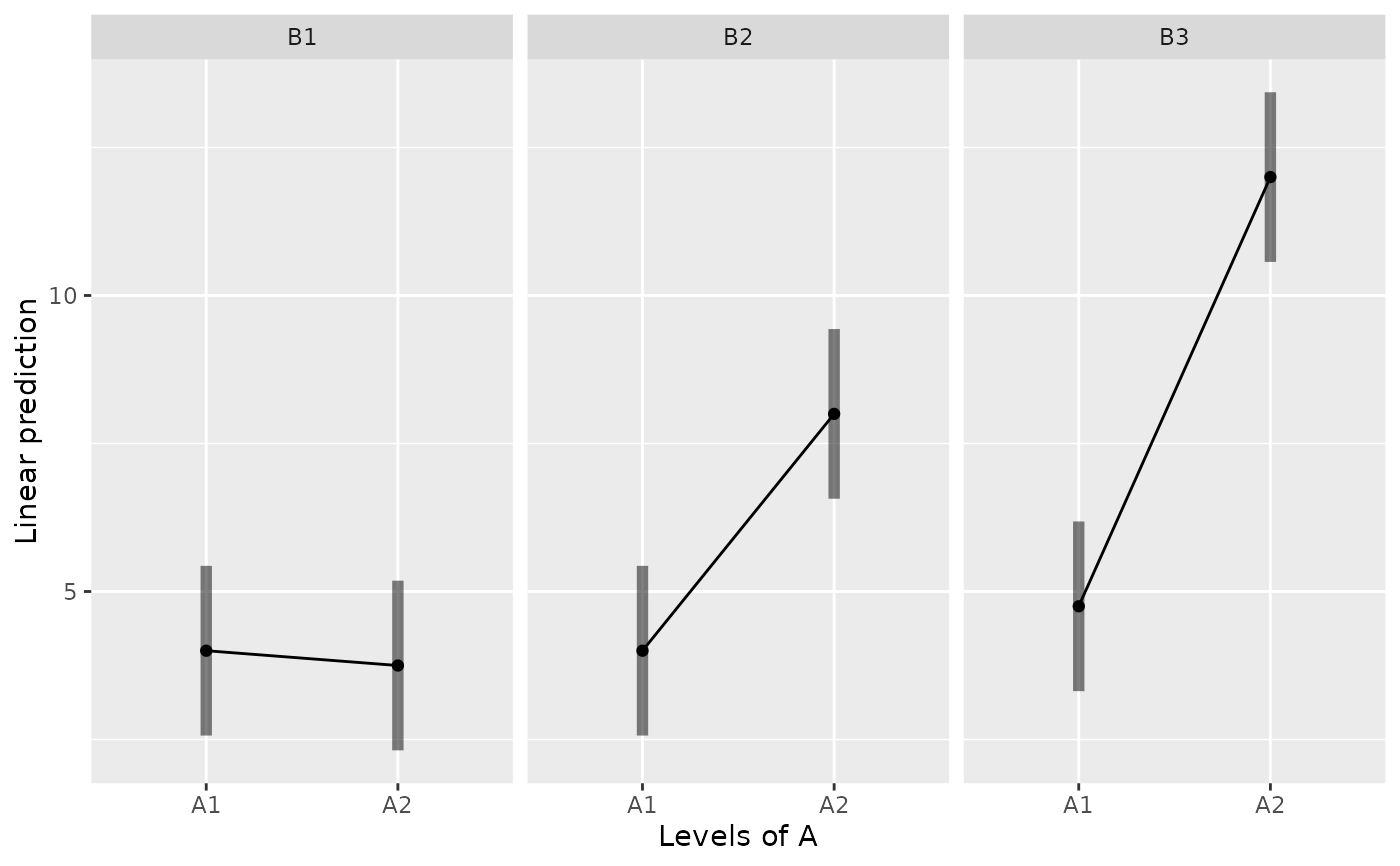
## How to create an interaction plot using `emmeans::emmip()`?
## See help page: ?emmeans::emmip()
m = MANOVA(between.2, dv="SCORE", between=c("A", "B"))
#> 
#> ====== ANOVA (Between-Subjects Design) ======
#> 
#> Descriptives:
#> ─────────────────────────
#>  "A" "B"   Mean    S.D. n
#> ─────────────────────────
#>   A1  B1  4.000 (1.414) 4
#>   A1  B2  4.000 (1.633) 4
#>   A1  B3  4.750 (2.062) 4
#>   A2  B1  3.750 (0.957) 4
#>   A2  B2  8.000 (0.816) 4
#>   A2  B3 12.000 (0.816) 4
#> ─────────────────────────
#> Total sample size: N = 24
#> 
#> ANOVA Table:
#> Dependent variable(s):      SCORE
#> Between-subjects factor(s): A, B
#> Within-subjects factor(s):  –
#> Covariate(s):               –
#> ─────────────────────────────────────────────────────────────────────
#>            MS   MSE df1 df2      F     p     η²p [90% CI of η²p]  η²G
#> ─────────────────────────────────────────────────────────────────────
#> A      80.667 1.861   1  18 43.343 <.001 ***   .707 [.482, .817] .707
#> B      40.542 1.861   2  18 21.784 <.001 ***   .708 [.470, .815] .708
#> A * B  28.292 1.861   2  18 15.201 <.001 ***   .628 [.347, .763] .628
#> ─────────────────────────────────────────────────────────────────────
#> MSE = mean square error (the residual variance of the linear model)
#> η²p = partial eta-squared = SS / (SS + SSE) = F * df1 / (F * df1 + df2)
#> ω²p = partial omega-squared = (F - 1) * df1 / (F * df1 + df2 + 1)
#> η²G = generalized eta-squared (see Olejnik & Algina, 2003)
#> Cohen’s f² = η²p / (1 - η²p)
#> 
#> Levene’s Test for Homogeneity of Variance:
#> ───────────────────────────────────────
#>            Levene’s F df1 df2     p    
#> ───────────────────────────────────────
#> DV: SCORE       0.605   5  18  .697    
#> ───────────────────────────────────────
#> 
emmip(m, ~ A | B, CIs=TRUE)

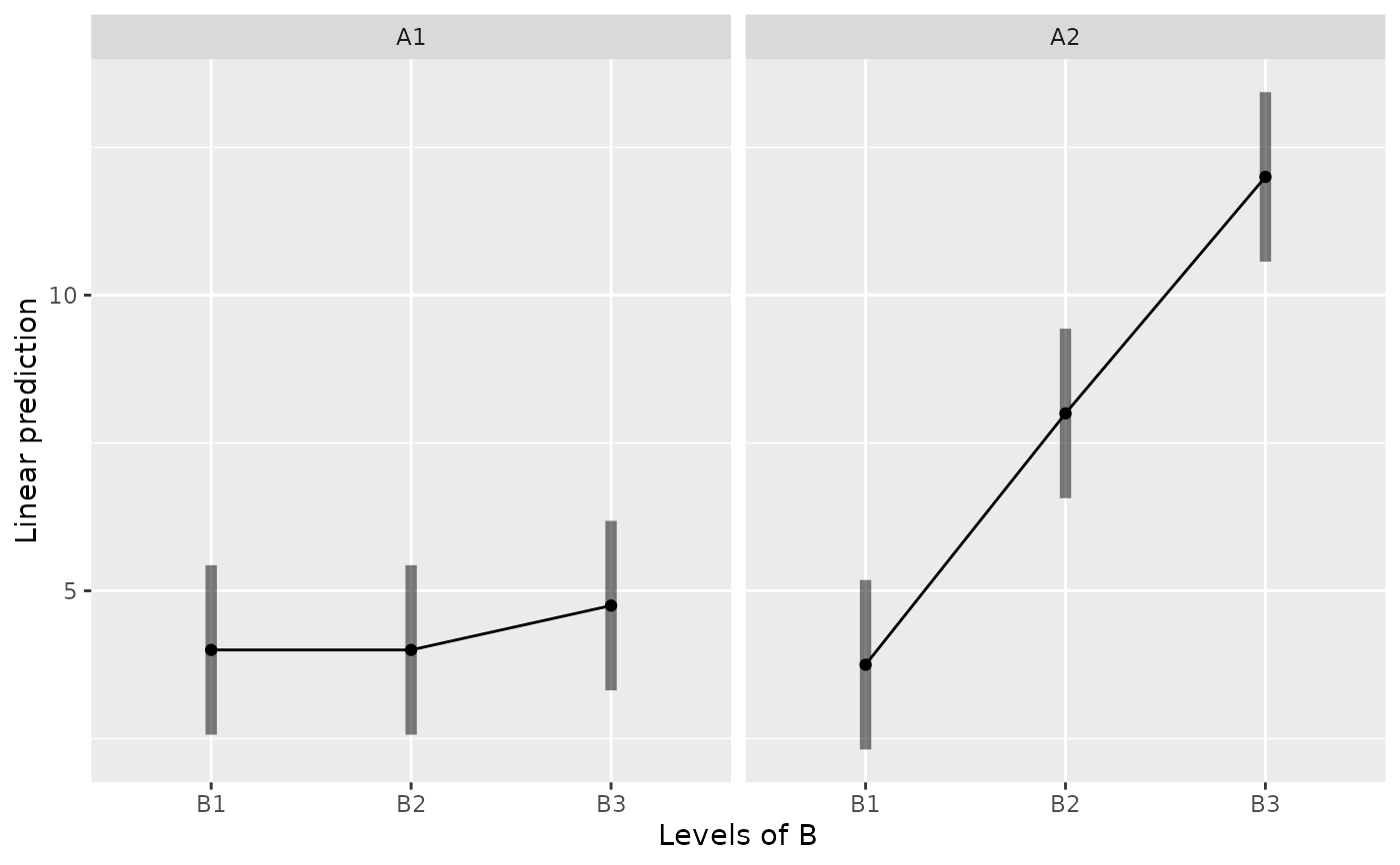
emmip(m, ~ B | A, CIs=TRUE)

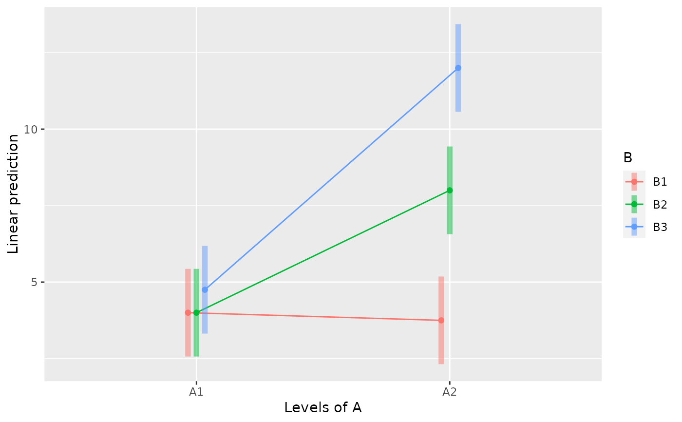
emmip(m, B ~ A, CIs=TRUE)

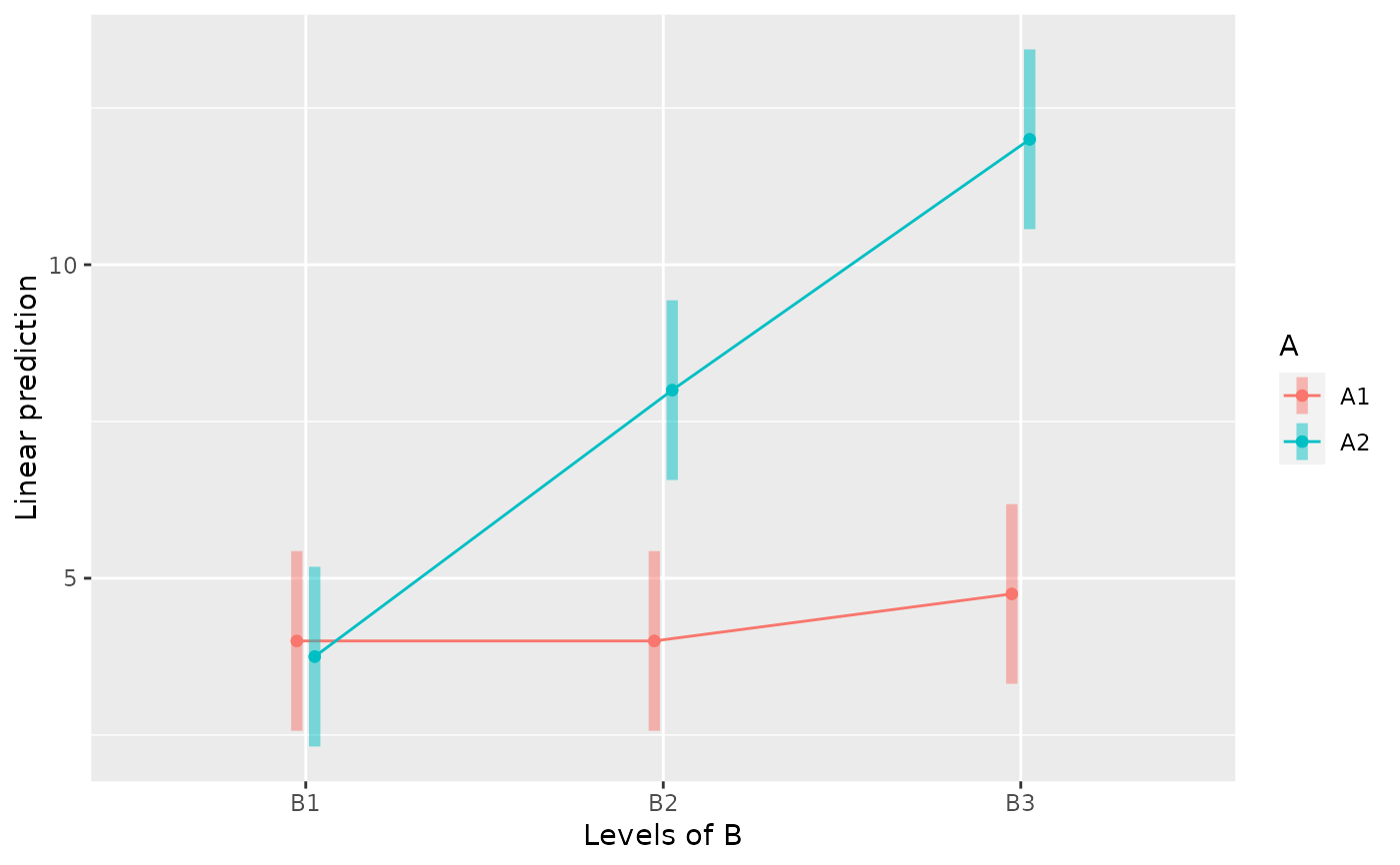
emmip(m, A ~ B, CIs=TRUE)


between.3
#>    A B C SCORE
#> 1  1 1 1     3
#> 2  1 1 1     6
#> 3  1 1 1     4
#> 4  1 1 1     3
#> 5  1 1 2     5
#> 6  1 1 2     7
#> 7  1 1 2     5
#> 8  1 1 2     2
#> 9  1 2 1     4
#> 10 1 2 1     6
#> 11 1 2 1     4
#> 12 1 2 1     2
#> 13 1 2 2     4
#> 14 1 2 2     5
#> 15 1 2 2     3
#> 16 1 2 2     3
#> 17 2 1 1     8
#> 18 2 1 1     9
#> 19 2 1 1     8
#> 20 2 1 1     7
#> 21 2 1 2     5
#> 22 2 1 2     6
#> 23 2 1 2     7
#> 24 2 1 2     6
#> 25 2 2 1     9
#> 26 2 2 1     8
#> 27 2 2 1     8
#> 28 2 2 1     7
#> 29 2 2 2    12
#> 30 2 2 2    13
#> 31 2 2 2    12
#> 32 2 2 2    11
MANOVA(between.3, dv="SCORE", between=c("A", "B", "C")) %>%
  EMMEANS("A", by="B") %>%
  EMMEANS(c("A", "B"), by="C") %>%
  EMMEANS("A", by=c("B", "C"))
#> 
#> ====== ANOVA (Between-Subjects Design) ======
#> 
#> Descriptives:
#> ─────────────────────────────
#>  "A" "B" "C"   Mean    S.D. n
#> ─────────────────────────────
#>   A1  B1  C1  4.000 (1.414) 4
#>   A1  B1  C2  4.750 (2.062) 4
#>   A1  B2  C1  4.000 (1.633) 4
#>   A1  B2  C2  3.750 (0.957) 4
#>   A2  B1  C1  8.000 (0.816) 4
#>   A2  B1  C2  6.000 (0.816) 4
#>   A2  B2  C1  8.000 (0.816) 4
#>   A2  B2  C2 12.000 (0.816) 4
#> ─────────────────────────────
#> Total sample size: N = 32
#> 
#> ANOVA Table:
#> Dependent variable(s):      SCORE
#> Between-subjects factor(s): A, B, C
#> Within-subjects factor(s):  –
#> Covariate(s):               –
#> ──────────────────────────────────────────────────────────────────────────
#>                 MS   MSE df1 df2      F     p     η²p [90% CI of η²p]  η²G
#> ──────────────────────────────────────────────────────────────────────────
#> A          153.125 1.563   1  24 98.000 <.001 ***   .803 [.670, .870] .803
#> B           12.500 1.563   1  24  8.000  .009 **    .250 [.042, .466] .250
#> C            3.125 1.563   1  24  2.000  .170       .077 [.000, .283] .077
#> A * B       24.500 1.563   1  24 15.680 <.001 ***   .395 [.147, .585] .395
#> A * C        1.125 1.563   1  24  0.720  .405       .029 [.000, .206] .029
#> B * C       12.500 1.563   1  24  8.000  .009 **    .250 [.042, .466] .250
#> A * B * C   24.500 1.563   1  24 15.680 <.001 ***   .395 [.147, .585] .395
#> ──────────────────────────────────────────────────────────────────────────
#> MSE = mean square error (the residual variance of the linear model)
#> η²p = partial eta-squared = SS / (SS + SSE) = F * df1 / (F * df1 + df2)
#> ω²p = partial omega-squared = (F - 1) * df1 / (F * df1 + df2 + 1)
#> η²G = generalized eta-squared (see Olejnik & Algina, 2003)
#> Cohen’s f² = η²p / (1 - η²p)
#> 
#> Levene’s Test for Homogeneity of Variance:
#> ───────────────────────────────────────
#>            Levene’s F df1 df2     p    
#> ───────────────────────────────────────
#> DV: SCORE       0.668   7  24  .697    
#> ───────────────────────────────────────
#> 
#> ------ EMMEANS (effect = "A") ------
#> 
#> Joint Tests of "A":
#> ────────────────────────────────────────────────────────
#>  Effect "B" df1 df2      F     p     η²p [90% CI of η²p]
#> ────────────────────────────────────────────────────────
#>   A      B1   1  24 17.640 <.001 ***   .424 [.173, .607]
#>   A      B2   1  24 96.040 <.001 ***   .800 [.665, .868]
#>   C      B1   1  24  1.000  .327       .040 [.000, .226]
#>   C      B2   1  24  9.000  .006 **    .273 [.055, .486]
#>   A * C  B1   1  24  4.840  .038 *     .168 [.006, .388]
#>   A * C  B2   1  24 11.560  .002 **    .325 [.090, .530]
#> ────────────────────────────────────────────────────────
#> Note. Simple effects of repeated measures with 3 or more levels
#> are different from the results obtained with SPSS MANOVA syntax.
#> 
#> Univariate Tests of "A":
#> ─────────────────────────────────────────────────────────
#>            Sum of Squares df Mean Square      F     p    
#> ─────────────────────────────────────────────────────────
#> B1: "A"            27.562  1      27.562 17.640 <.001 ***
#> B2: "A"           150.062  1     150.062 96.040 <.001 ***
#> Residuals          37.500 24       1.563                 
#> ─────────────────────────────────────────────────────────
#> Note. Identical to the results obtained with SPSS GLM EMMEANS syntax.
#> 
#> Estimated Marginal Means of "A":
#> ───────────────────────────────────────
#>  "A" "B"  Mean [95% CI of Mean]    S.E.
#> ───────────────────────────────────────
#>   A1  B1  4.375 [3.463,  5.287] (0.442)
#>   A2  B1  7.000 [6.088,  7.912] (0.442)
#>   A1  B2  3.875 [2.963,  4.787] (0.442)
#>   A2  B2 10.000 [9.088, 10.912] (0.442)
#> ───────────────────────────────────────
#> 
#> Pairwise Comparisons of "A":
#> ─────────────────────────────────────────────────────────────────────────
#>  Contrast "B" Estimate    S.E. df     t     p     Cohen’s d [95% CI of d]
#> ─────────────────────────────────────────────────────────────────────────
#>   A2 - A1  B1    2.625 (0.625) 24 4.200 <.001 ***    2.100 [1.068, 3.132]
#>   A2 - A1  B2    6.125 (0.625) 24 9.800 <.001 ***    4.900 [3.868, 5.932]
#> ─────────────────────────────────────────────────────────────────────────
#> Pooled SD for computing Cohen’s d: 1.250
#> Results are averaged over the levels of: C
#> No need to adjust p values.
#> 
#> Disclaimer:
#> By default, pooled SD is Root Mean Square Error (RMSE).
#> There is much disagreement on how to compute Cohen’s d.
#> You are completely responsible for setting `sd.pooled`.
#> You might also use `effectsize::t_to_d()` to compute d.
#> 
#> ------ EMMEANS (effect = "A" & "B") ------
#> 
#> Joint Tests of "A" & "B":
#> ────────────────────────────────────────────────────────
#>  Effect "C" df1 df2      F     p     η²p [90% CI of η²p]
#> ────────────────────────────────────────────────────────
#>   A      C1   1  24 40.960 <.001 ***   .631 [.414, .754]
#>   A      C2   1  24 57.760 <.001 ***   .706 [.521, .806]
#>   B      C1   1  24  0.000 1.000       .000 [.000, .000]
#>   B      C2   1  24 16.000 <.001 ***   .400 [.151, .589]
#>   A * B  C1   1  24  0.000 1.000       .000 [.000, .000]
#>   A * B  C2   1  24 31.360 <.001 ***   .566 [.331, .710]
#> ────────────────────────────────────────────────────────
#> Note. Simple effects of repeated measures with 3 or more levels
#> are different from the results obtained with SPSS MANOVA syntax.
#> 
#> Univariate Tests of "A" & "B":
#> ─────────────────────────────────────────────────────────────
#>                Sum of Squares df Mean Square      F     p    
#> ─────────────────────────────────────────────────────────────
#> C1: "A" & "B"           0.000  1       0.000  0.000 1.000    
#> C2: "A" & "B"          49.000  1      49.000 31.360 <.001 ***
#> Residuals              37.500 24       1.563                 
#> ─────────────────────────────────────────────────────────────
#> Note. Identical to the results obtained with SPSS GLM EMMEANS syntax.
#> 
#> Estimated Marginal Means of "A" & "B":
#> ────────────────────────────────────────
#>  "A" "B"   Mean [95% CI of Mean]    S.E.
#> ────────────────────────────────────────
#>   A1  B1  4.000 [ 2.710,  5.290] (0.625)
#>   A2  B1  8.000 [ 6.710,  9.290] (0.625)
#>   A1  B2  4.000 [ 2.710,  5.290] (0.625)
#>   A2  B2  8.000 [ 6.710,  9.290] (0.625)
#>   A1  B1  4.750 [ 3.460,  6.040] (0.625)
#>   A2  B1  6.000 [ 4.710,  7.290] (0.625)
#>   A1  B2  3.750 [ 2.460,  5.040] (0.625)
#>   A2  B2 12.000 [10.710, 13.290] (0.625)
#> ────────────────────────────────────────
#> 
#> Pairwise Comparisons of "A" & "B":
#> ───────────────────────────────────────────────────────────────────────────────
#>       Contrast "C" Estimate    S.E. df      t     p     Cohen’s d [95% CI of d]
#> ───────────────────────────────────────────────────────────────────────────────
#>  A2 B1 - A1 B1  C1    4.000 (0.884) 24  4.525 <.001 ***  3.200 [ 1.167,  5.233]
#>  A1 B2 - A1 B1  C1   -0.000 (0.884) 24 -0.000 1.000     -0.000 [-2.033,  2.033]
#>  A1 B2 - A2 B1  C1   -4.000 (0.884) 24 -4.525 <.001 *** -3.200 [-5.233, -1.167]
#>  A2 B2 - A1 B1  C1    4.000 (0.884) 24  4.525 <.001 ***  3.200 [ 1.167,  5.233]
#>  A2 B2 - A2 B1  C1   -0.000 (0.884) 24 -0.000 1.000     -0.000 [-2.033,  2.033]
#>  A2 B2 - A1 B2  C1    4.000 (0.884) 24  4.525 <.001 ***  3.200 [ 1.167,  5.233]
#>  A2 B1 - A1 B1  C2    1.250 (0.884) 24  1.414 1.000      1.000 [-1.033,  3.033]
#>  A1 B2 - A1 B1  C2   -1.000 (0.884) 24 -1.131 1.000     -0.800 [-2.833,  1.233]
#>  A1 B2 - A2 B1  C2   -2.250 (0.884) 24 -2.546  .107     -1.800 [-3.833,  0.233]
#>  A2 B2 - A1 B1  C2    7.250 (0.884) 24  8.202 <.001 ***  5.800 [ 3.767,  7.833]
#>  A2 B2 - A2 B1  C2    6.000 (0.884) 24  6.788 <.001 ***  4.800 [ 2.767,  6.833]
#>  A2 B2 - A1 B2  C2    8.250 (0.884) 24  9.334 <.001 ***  6.600 [ 4.567,  8.633]
#> ───────────────────────────────────────────────────────────────────────────────
#> Pooled SD for computing Cohen’s d: 1.250
#> P-value adjustment: Bonferroni method for 6 tests.
#> 
#> Disclaimer:
#> By default, pooled SD is Root Mean Square Error (RMSE).
#> There is much disagreement on how to compute Cohen’s d.
#> You are completely responsible for setting `sd.pooled`.
#> You might also use `effectsize::t_to_d()` to compute d.
#> 
#> ------ EMMEANS (effect = "A") ------
#> 
#> Joint Tests of "A":
#> ────────────────────────────────────────────────────────────
#>  Effect "B" "C" df1 df2      F     p     η²p [90% CI of η²p]
#> ────────────────────────────────────────────────────────────
#>       A  B1  C1   1  24 20.480 <.001 ***   .460 [.210, .634]
#>       A  B2  C1   1  24 20.480 <.001 ***   .460 [.210, .634]
#>       A  B1  C2   1  24  2.000  .170       .077 [.000, .283]
#>       A  B2  C2   1  24 87.120 <.001 ***   .784 [.639, .858]
#> ────────────────────────────────────────────────────────────
#> Note. Simple effects of repeated measures with 3 or more levels
#> are different from the results obtained with SPSS MANOVA syntax.
#> 
#> Univariate Tests of "A":
#> ────────────────────────────────────────────────────────────
#>               Sum of Squares df Mean Square      F     p    
#> ────────────────────────────────────────────────────────────
#> B1 & C1: "A"          32.000  1      32.000 20.480 <.001 ***
#> B2 & C1: "A"          32.000  1      32.000 20.480 <.001 ***
#> B1 & C2: "A"           3.125  1       3.125  2.000  .170    
#> B2 & C2: "A"         136.125  1     136.125 87.120 <.001 ***
#> Residuals             37.500 24       1.563                 
#> ────────────────────────────────────────────────────────────
#> Note. Identical to the results obtained with SPSS GLM EMMEANS syntax.
#> 
#> Estimated Marginal Means of "A":
#> ────────────────────────────────────────────
#>  "A" "B" "C"   Mean [95% CI of Mean]    S.E.
#> ────────────────────────────────────────────
#>   A1  B1  C1  4.000 [ 2.710,  5.290] (0.625)
#>   A2  B1  C1  8.000 [ 6.710,  9.290] (0.625)
#>   A1  B2  C1  4.000 [ 2.710,  5.290] (0.625)
#>   A2  B2  C1  8.000 [ 6.710,  9.290] (0.625)
#>   A1  B1  C2  4.750 [ 3.460,  6.040] (0.625)
#>   A2  B1  C2  6.000 [ 4.710,  7.290] (0.625)
#>   A1  B2  C2  3.750 [ 2.460,  5.040] (0.625)
#>   A2  B2  C2 12.000 [10.710, 13.290] (0.625)
#> ────────────────────────────────────────────
#> 
#> Pairwise Comparisons of "A":
#> ─────────────────────────────────────────────────────────────────────────────
#>  Contrast "B" "C" Estimate    S.E. df     t     p     Cohen’s d [95% CI of d]
#> ─────────────────────────────────────────────────────────────────────────────
#>   A2 - A1  B1  C1    4.000 (0.884) 24 4.525 <.001 ***   3.200 [ 1.741, 4.659]
#>   A2 - A1  B2  C1    4.000 (0.884) 24 4.525 <.001 ***   3.200 [ 1.741, 4.659]
#>   A2 - A1  B1  C2    1.250 (0.884) 24 1.414  .170       1.000 [-0.459, 2.459]
#>   A2 - A1  B2  C2    8.250 (0.884) 24 9.334 <.001 ***   6.600 [ 5.141, 8.059]
#> ─────────────────────────────────────────────────────────────────────────────
#> Pooled SD for computing Cohen’s d: 1.250
#> No need to adjust p values.
#> 
#> Disclaimer:
#> By default, pooled SD is Root Mean Square Error (RMSE).
#> There is much disagreement on how to compute Cohen’s d.
#> You are completely responsible for setting `sd.pooled`.
#> You might also use `effectsize::t_to_d()` to compute d.
#> 
## Just to name a few...
## You may test other combinations...


#### Within-Subjects Design ####

within.1
#>   ID A1 A2 A3 A4
#> 1 S1  3  4  8  9
#> 2 S2  6  6  9  8
#> 3 S3  4  4  8  8
#> 4 S4  3  2  7  7
#> 5 S5  5  4  5 12
#> 6 S6  7  5  6 13
#> 7 S7  5  3  7 12
#> 8 S8  2  3  6 11
MANOVA(within.1, dvs="A1:A4", dvs.pattern="A(.)",
       within="A") %>%
  EMMEANS("A")
#> 
#> Note:
#> dvs="A1:A4" is matched to variables:
#> A1, A2, A3, A4
#> 
#> ====== ANOVA (Within-Subjects Design) ======
#> 
#> Descriptives:
#> ─────────────────────
#>  "A"   Mean    S.D. n
#> ─────────────────────
#>   A1  4.375 (1.685) 8
#>   A2  3.875 (1.246) 8
#>   A3  7.000 (1.309) 8
#>   A4 10.000 (2.268) 8
#> ─────────────────────
#> Total sample size: N = 8
#> 
#> ANOVA Table:
#> Dependent variable(s):      A1, A2, A3, A4
#> Between-subjects factor(s): –
#> Within-subjects factor(s):  A
#> Covariate(s):               –
#> ─────────────────────────────────────────────────────────────────
#>        MS   MSE df1 df2      F     p     η²p [90% CI of η²p]  η²G
#> ─────────────────────────────────────────────────────────────────
#> A  63.375 2.518   3  21 25.170 <.001 ***   .782 [.609, .858] .707
#> ─────────────────────────────────────────────────────────────────
#> MSE = mean square error (the residual variance of the linear model)
#> η²p = partial eta-squared = SS / (SS + SSE) = F * df1 / (F * df1 + df2)
#> ω²p = partial omega-squared = (F - 1) * df1 / (F * df1 + df2 + 1)
#> η²G = generalized eta-squared (see Olejnik & Algina, 2003)
#> Cohen’s f² = η²p / (1 - η²p)
#> 
#> Levene’s Test for Homogeneity of Variance:
#> No between-subjects factors. No need to do the Levene’s test.
#> 
#> Mauchly’s Test of Sphericity:
#> ────────────────────────
#>    Mauchly's W     p    
#> ────────────────────────
#> A       0.1899  .095 .  
#> ────────────────────────
#> 
#> ------ EMMEANS (effect = "A") ------
#> 
#> Joint Tests of "A":
#> ────────────────────────────────────────────────────
#>  Effect df1 df2      F     p     η²p [90% CI of η²p]
#> ────────────────────────────────────────────────────
#>       A   3   7 47.960 <.001 ***   .954 [.848, .977]
#> ────────────────────────────────────────────────────
#> Note. Simple effects of repeated measures with 3 or more levels
#> are different from the results obtained with SPSS MANOVA syntax.
#> 
#> Multivariate Tests of "A":
#> ───────────────────────────────────────────────────────────────
#>            Pillai’s trace Hypoth. df Error df Exact F     p    
#> ───────────────────────────────────────────────────────────────
#> Mean: "A"           0.954      3.000    5.000  34.257 <.001 ***
#> ───────────────────────────────────────────────────────────────
#> Note. Identical to the results obtained with SPSS GLM EMMEANS syntax.
#> 
#> Estimated Marginal Means of "A":
#> ───────────────────────────────────
#>  "A"  Mean [95% CI of Mean]    S.E.
#> ───────────────────────────────────
#>   A1  4.375 [2.966,  5.784] (0.596)
#>   A2  3.875 [2.833,  4.917] (0.441)
#>   A3  7.000 [5.905,  8.095] (0.463)
#>   A4 10.000 [8.104, 11.896] (0.802)
#> ───────────────────────────────────
#> 
#> Pairwise Comparisons of "A":
#> ──────────────────────────────────────────────────────────────────────
#>  Contrast Estimate    S.E. df      t     p     Cohen’s d [95% CI of d]
#> ──────────────────────────────────────────────────────────────────────
#>   A2 - A1   -0.500 (0.423)  7 -1.183 1.000      -0.223 [-0.907, 0.462]
#>   A3 - A1    2.625 (0.754)  7  3.479  .062 .     1.170 [-0.053, 2.392]
#>   A3 - A2    3.125 (0.515)  7  6.063  .003 **    1.393 [ 0.558, 2.228]
#>   A4 - A1    5.625 (0.778)  7  7.232  .001 **    2.507 [ 1.247, 3.767]
#>   A4 - A2    6.125 (0.875)  7  7.000  .001 **    2.729 [ 1.312, 4.147]
#>   A4 - A3    3.000 (1.180)  7  2.542  .231       1.337 [-0.575, 3.249]
#> ──────────────────────────────────────────────────────────────────────
#> Pooled SD for computing Cohen’s d: 2.244
#> P-value adjustment: Bonferroni method for 6 tests.
#> 
#> Disclaimer:
#> By default, pooled SD is Root Mean Square Error (RMSE).
#> There is much disagreement on how to compute Cohen’s d.
#> You are completely responsible for setting `sd.pooled`.
#> You might also use `effectsize::t_to_d()` to compute d.
#> 

within.2
#>   ID A1B1 A1B2 A1B3 A2B1 A2B2 A2B3
#> 1 S1    3    4    5    4    8   12
#> 2 S2    6    6    7    5    9   13
#> 3 S3    4    4    5    3    8   12
#> 4 S4    3    2    2    3    7   11
MANOVA(within.2, dvs="A1B1:A2B3", dvs.pattern="A(.)B(.)",
       within=c("A", "B")) %>%
  EMMEANS("A", by="B") %>%
  EMMEANS("B", by="A")  # singular error matrix
#> 
#> Note:
#> dvs="A1B1:A2B3" is matched to variables:
#> A1B1, A1B2, A1B3, A2B1, A2B2, A2B3
#> 
#> ====== ANOVA (Within-Subjects Design) ======
#> 
#> Descriptives:
#> ─────────────────────────
#>  "A" "B"   Mean    S.D. n
#> ─────────────────────────
#>   A1  B1  4.000 (1.414) 4
#>   A1  B2  4.000 (1.633) 4
#>   A1  B3  4.750 (2.062) 4
#>   A2  B1  3.750 (0.957) 4
#>   A2  B2  8.000 (0.816) 4
#>   A2  B3 12.000 (0.816) 4
#> ─────────────────────────
#> Total sample size: N = 4
#> 
#> ANOVA Table:
#> Dependent variable(s):      A1B1, A1B2, A1B3, A2B1, A2B2, A2B3
#> Between-subjects factor(s): –
#> Within-subjects factor(s):  A, B
#> Covariate(s):               –
#> ──────────────────────────────────────────────────────────────────────
#>            MS   MSE df1 df2       F     p     η²p [90% CI of η²p]  η²G
#> ──────────────────────────────────────────────────────────────────────
#> A      80.667 1.111   1   3  72.600  .003 **    .960 [.699, .985] .707
#> B      40.542 0.264   2   6 153.632 <.001 ***   .981 [.930, .991] .708
#> A * B  28.292 0.236   2   6 119.824 <.001 ***   .976 [.911, .988] .628
#> ──────────────────────────────────────────────────────────────────────
#> MSE = mean square error (the residual variance of the linear model)
#> η²p = partial eta-squared = SS / (SS + SSE) = F * df1 / (F * df1 + df2)
#> ω²p = partial omega-squared = (F - 1) * df1 / (F * df1 + df2 + 1)
#> η²G = generalized eta-squared (see Olejnik & Algina, 2003)
#> Cohen’s f² = η²p / (1 - η²p)
#> 
#> Levene’s Test for Homogeneity of Variance:
#> No between-subjects factors. No need to do the Levene’s test.
#> 
#> Mauchly’s Test of Sphericity:
#> ────────────────────────────
#>        Mauchly's W     p    
#> ────────────────────────────
#> B           0.0665  .066 .  
#> A * B       0.2491  .249    
#> ────────────────────────────
#> 
#> ------ EMMEANS (effect = "A") ------
#> 
#> Joint Tests of "A":
#> ─────────────────────────────────────────────────────────
#>  Effect "B" df1 df2       F     p     η²p [90% CI of η²p]
#> ─────────────────────────────────────────────────────────
#>       A  B1   1   3   0.273  .638       .083 [.000, .597]
#>       A  B2   1   3  96.000  .002 **    .970 [.763, .988]
#>       A  B3   1   3 132.789  .001 **    .978 [.823, .992]
#> ─────────────────────────────────────────────────────────
#> Note. Simple effects of repeated measures with 3 or more levels
#> are different from the results obtained with SPSS MANOVA syntax.
#> 
#> Multivariate Tests of "A":
#> ─────────────────────────────────────────────────────────────
#>          Pillai’s trace Hypoth. df Error df Exact F     p    
#> ─────────────────────────────────────────────────────────────
#> B1: "A"           0.083      1.000    3.000   0.273  .638    
#> B2: "A"           0.970      1.000    3.000  96.000  .002 ** 
#> B3: "A"           0.978      1.000    3.000 132.789  .001 ** 
#> ─────────────────────────────────────────────────────────────
#> Note. Identical to the results obtained with SPSS GLM EMMEANS syntax.
#> 
#> Estimated Marginal Means of "A":
#> ────────────────────────────────────────
#>  "A" "B"   Mean [95% CI of Mean]    S.E.
#> ────────────────────────────────────────
#>   A1  B1  4.000 [ 1.750,  6.250] (0.707)
#>   A2  B1  3.750 [ 2.227,  5.273] (0.479)
#>   A1  B2  4.000 [ 1.402,  6.598] (0.816)
#>   A2  B2  8.000 [ 6.701,  9.299] (0.408)
#>   A1  B3  4.750 [ 1.470,  8.030] (1.031)
#>   A2  B3 12.000 [10.701, 13.299] (0.408)
#> ────────────────────────────────────────
#> 
#> Pairwise Comparisons of "A":
#> ──────────────────────────────────────────────────────────────────────────
#>  Contrast "B" Estimate    S.E. df      t     p     Cohen’s d [95% CI of d]
#> ──────────────────────────────────────────────────────────────────────────
#>   A2 - A1  B1   -0.250 (0.479)  3 -0.522  .638     -0.272 [-1.930,  1.386]
#>   A2 - A1  B2    4.000 (0.408)  3  9.798  .002 **   4.353 [ 2.939,  5.767]
#>   A2 - A1  B3    7.250 (0.629)  3 11.523  .001 **   7.890 [ 5.711, 10.068]
#> ──────────────────────────────────────────────────────────────────────────
#> Pooled SD for computing Cohen’s d: 0.919
#> No need to adjust p values.
#> 
#> Disclaimer:
#> By default, pooled SD is Root Mean Square Error (RMSE).
#> There is much disagreement on how to compute Cohen’s d.
#> You are completely responsible for setting `sd.pooled`.
#> You might also use `effectsize::t_to_d()` to compute d.
#> 
#> ------ EMMEANS (effect = "B") ------
#> 
#> Error in solve.default(zcov, z) : 
#>   system is computationally singular: reciprocal condition number = 2.23113e-17
#> Error in solve.default(zcov, z) : 
#>   system is computationally singular: reciprocal condition number = 2.23113e-17
#> Warning: Some CIs could not be estimated due to non-finite F, df, or df_error
#>   values.
#> Joint Tests of "B":
#> ───────────────────────────────────────────────────────────────
#>        Effect "A" df1 df2      F     p      η²p [90% CI of η²p]
#> ───────────────────────────────────────────────────────────────
#>  B             A1   2   3 13.500  .032 *   .900 [.219, .962]   
#>  B             A2   2                         NA [   NA,    NA]
#>  (confounded)  A2   2                         NA [   NA,    NA]
#> ───────────────────────────────────────────────────────────────
#> Note. Simple effects of repeated measures with 3 or more levels
#> are different from the results obtained with SPSS MANOVA syntax.
#> 
#> Estimated Marginal Means of "B":
#> ────────────────────────────────────────
#>  "B" "A"   Mean [95% CI of Mean]    S.E.
#> ────────────────────────────────────────
#>   B1  A1  4.000 [ 1.750,  6.250] (0.707)
#>   B2  A1  4.000 [ 1.402,  6.598] (0.816)
#>   B3  A1  4.750 [ 1.470,  8.030] (1.031)
#>   B1  A2  3.750 [ 2.227,  5.273] (0.479)
#>   B2  A2  8.000 [ 6.701,  9.299] (0.408)
#>   B3  A2 12.000 [10.701, 13.299] (0.408)
#> ────────────────────────────────────────
#> 
#> Pairwise Comparisons of "B":
#> ──────────────────────────────────────────────────────────────────────────
#>  Contrast "A" Estimate    S.E. df      t     p     Cohen’s d [95% CI of d]
#> ──────────────────────────────────────────────────────────────────────────
#>   B2 - B1  A1    0.000 (0.408)  3  0.000 1.000      0.000 [-2.158,  2.158]
#>   B3 - B1  A1    0.750 (0.629)  3  1.192  .957      0.816 [-2.509,  4.141]
#>   B3 - B2  A1    0.750 (0.250)  3  3.000  .173      0.816 [-0.505,  2.137]
#>   B2 - B1  A2    4.250 (0.250)  3 17.000  .001 **   4.625 [ 3.304,  5.946]
#>   B3 - B1  A2    8.250 (0.250)  3 33.000 <.001 ***  8.978 [ 7.656, 10.299]
#>   B3 - B2  A2    4.000 (0.000)  3    Inf <.001 ***  4.353 [ 4.353,  4.353]
#> ──────────────────────────────────────────────────────────────────────────
#> Pooled SD for computing Cohen’s d: 0.919
#> P-value adjustment: Bonferroni method for 3 tests.
#> 
#> Disclaimer:
#> By default, pooled SD is Root Mean Square Error (RMSE).
#> There is much disagreement on how to compute Cohen’s d.
#> You are completely responsible for setting `sd.pooled`.
#> You might also use `effectsize::t_to_d()` to compute d.
#> 
# :::::::::::::::::::::::::::::::::::::::
# This would produce a WARNING because of
# the linear dependence of A2B2 and A2B3.
# See: Corr(within.2[c("A2B2", "A2B3")])

within.3
#>   ID A1B1C1 A1B1C2 A1B2C1 A1B2C2 A2B1C1 A2B1C2 A2B2C1 A2B2C2
#> 1 S1      3      5      4      4      8      5      9     12
#> 2 S2      6      7      6      5      9      6      8     13
#> 3 S3      4      5      4      3      8      7      8     12
#> 4 S4      3      2      2      3      7      6      7     11
MANOVA(within.3, dvs="A1B1C1:A2B2C2", dvs.pattern="A(.)B(.)C(.)",
       within=c("A", "B", "C")) %>%
  EMMEANS("A", by="B") %>%
  EMMEANS(c("A", "B"), by="C") %>%
  EMMEANS("A", by=c("B", "C"))
#> 
#> Note:
#> dvs="A1B1C1:A2B2C2" is matched to variables:
#> A1B1C1, A1B1C2, A1B2C1, A1B2C2, A2B1C1, A2B1C2, A2B2C1, A2B2C2
#> 
#> ====== ANOVA (Within-Subjects Design) ======
#> 
#> Descriptives:
#> ─────────────────────────────
#>  "A" "B" "C"   Mean    S.D. n
#> ─────────────────────────────
#>   A1  B1  C1  4.000 (1.414) 4
#>   A1  B1  C2  4.750 (2.062) 4
#>   A1  B2  C1  4.000 (1.633) 4
#>   A1  B2  C2  3.750 (0.957) 4
#>   A2  B1  C1  8.000 (0.816) 4
#>   A2  B1  C2  6.000 (0.816) 4
#>   A2  B2  C1  8.000 (0.816) 4
#>   A2  B2  C2 12.000 (0.816) 4
#> ─────────────────────────────
#> Total sample size: N = 4
#> 
#> ANOVA Table:
#> Dependent variable(s):      A1B1C1, A1B1C2, A1B2C1, A1B2C2, A2B1C1, A2B1C2, A2B2C1, A2B2C2
#> Between-subjects factor(s): –
#> Within-subjects factor(s):  A, B, C
#> Covariate(s):               –
#> ──────────────────────────────────────────────────────────────────────────
#>                 MS   MSE df1 df2      F     p     η²p [90% CI of η²p]  η²G
#> ──────────────────────────────────────────────────────────────────────────
#> A          153.125 1.875   1   3 81.667  .003 **    .965 [.727, .986] .803
#> B           12.500 0.583   1   3 21.429  .019 *     .877 [.279, .954] .250
#> C            3.125 0.042   1   3 75.000  .003 **    .962 [.707, .985] .077
#> A * B       24.500 0.250   1   3 98.000  .002 **    .970 [.768, .989] .395
#> A * C        1.125 0.708   1   3  1.588  .297       .346 [.000, .751] .029
#> B * C       12.500 0.417   1   3 30.000  .012 *     .909 [.411, .965] .250
#> A * B * C   24.500 1.083   1   3 22.615  .018 *     .883 [.300, .956] .395
#> ──────────────────────────────────────────────────────────────────────────
#> MSE = mean square error (the residual variance of the linear model)
#> η²p = partial eta-squared = SS / (SS + SSE) = F * df1 / (F * df1 + df2)
#> ω²p = partial omega-squared = (F - 1) * df1 / (F * df1 + df2 + 1)
#> η²G = generalized eta-squared (see Olejnik & Algina, 2003)
#> Cohen’s f² = η²p / (1 - η²p)
#> 
#> Levene’s Test for Homogeneity of Variance:
#> No between-subjects factors. No need to do the Levene’s test.
#> 
#> Mauchly’s Test of Sphericity:
#> The repeated measures have only two levels. The assumption of sphericity is always met.
#> 
#> ------ EMMEANS (effect = "A") ------
#> 
#> Joint Tests of "A":
#> ─────────────────────────────────────────────────────────
#>  Effect "B" df1 df2       F     p     η²p [90% CI of η²p]
#> ─────────────────────────────────────────────────────────
#>   C      B1   1   3   6.818  .080 .     .694 [.000, .886]
#>   C      B2   1   3  61.364  .004 **    .953 [.653, .982]
#>   A      B1   1   3  17.640  .025 *     .855 [.202, .945]
#>   A      B2   1   3 266.778 <.001 ***   .989 [.908, .996]
#>   C * A  B1   1   3   6.153  .089 .     .672 [.000, .877]
#>   C * A  B2   1   3  32.111  .011 *     .915 [.436, .968]
#> ─────────────────────────────────────────────────────────
#> Note. Simple effects of repeated measures with 3 or more levels
#> are different from the results obtained with SPSS MANOVA syntax.
#> 
#> Multivariate Tests of "A":
#> ─────────────────────────────────────────────────────────────
#>          Pillai’s trace Hypoth. df Error df Exact F     p    
#> ─────────────────────────────────────────────────────────────
#> B1: "A"           0.855      1.000    3.000  17.640  .025 *  
#> B2: "A"           0.989      1.000    3.000 266.778 <.001 ***
#> ─────────────────────────────────────────────────────────────
#> Note. Identical to the results obtained with SPSS GLM EMMEANS syntax.
#> 
#> Estimated Marginal Means of "A":
#> ───────────────────────────────────────
#>  "A" "B"  Mean [95% CI of Mean]    S.E.
#> ───────────────────────────────────────
#>   A1  B1  4.375 [1.746,  7.004] (0.826)
#>   A2  B1  7.000 [6.081,  7.919] (0.289)
#>   A1  B2  3.875 [1.886,  5.864] (0.625)
#>   A2  B2 10.000 [8.875, 11.125] (0.354)
#> ───────────────────────────────────────
#> 
#> Pairwise Comparisons of "A":
#> ──────────────────────────────────────────────────────────────────────────
#>  Contrast "B" Estimate    S.E. df      t     p     Cohen’s d [95% CI of d]
#> ──────────────────────────────────────────────────────────────────────────
#>   A2 - A1  B1    2.625 (0.625)  3  4.200  .025 *      2.205 [0.534, 3.877]
#>   A2 - A1  B2    6.125 (0.375)  3 16.333 <.001 ***    5.146 [4.143, 6.149]
#> ──────────────────────────────────────────────────────────────────────────
#> Pooled SD for computing Cohen’s d: 1.190
#> Results are averaged over the levels of: C
#> No need to adjust p values.
#> 
#> Disclaimer:
#> By default, pooled SD is Root Mean Square Error (RMSE).
#> There is much disagreement on how to compute Cohen’s d.
#> You are completely responsible for setting `sd.pooled`.
#> You might also use `effectsize::t_to_d()` to compute d.
#> 
#> ------ EMMEANS (effect = "A" & "B") ------
#> 
#> Error in solve.default(zcov, z) : 
#>   system is computationally singular: reciprocal condition number = 3.3515e-17
#> Error in solve.default(zcov, z) : 
#>   system is computationally singular: reciprocal condition number = 1.38778e-17
#> Joint Tests of "A" & "B":
#> ────────────────────────────────────────────────────────
#>  Effect "C" df1 df2      F     p     η²p [90% CI of η²p]
#> ────────────────────────────────────────────────────────
#>   B      C1   1   3  0.000 1.000       .000 [.000, .000]
#>   B      C2   1   3 50.000  .006 **    .943 [.610, .978]
#>   A      C1   1   3 54.857  .005 **    .948 [.620, .980]
#>   A      C2   1   3 63.706  .004 **    .955 [.664, .983]
#>   B * A  C1   1   3  0.000 1.000       .000 [.000, .000]
#>   B * A  C2   1   3 42.000  .007 **    .933 [.534, .975]
#> ────────────────────────────────────────────────────────
#> Note. Simple effects of repeated measures with 3 or more levels
#> are different from the results obtained with SPSS MANOVA syntax.
#> 
#> Multivariate Tests of "A" & "B":
#> ───────────────────────────────────────────────────────────────────
#>                Pillai’s trace Hypoth. df Error df Exact F     p    
#> ───────────────────────────────────────────────────────────────────
#> C1: "A" & "B"           0.000      1.000    3.000   0.000 1.000    
#> C2: "A" & "B"           0.933      1.000    3.000  42.000  .007 ** 
#> ───────────────────────────────────────────────────────────────────
#> Note. Identical to the results obtained with SPSS GLM EMMEANS syntax.
#> 
#> Estimated Marginal Means of "A" & "B":
#> ────────────────────────────────────────
#>  "A" "B"   Mean [95% CI of Mean]    S.E.
#> ────────────────────────────────────────
#>   A1  B1  4.000 [ 1.750,  6.250] (0.707)
#>   A2  B1  8.000 [ 6.701,  9.299] (0.408)
#>   A1  B2  4.000 [ 1.402,  6.598] (0.816)
#>   A2  B2  8.000 [ 6.701,  9.299] (0.408)
#>   A1  B1  4.750 [ 1.470,  8.030] (1.031)
#>   A2  B1  6.000 [ 4.701,  7.299] (0.408)
#>   A1  B2  3.750 [ 2.227,  5.273] (0.479)
#>   A2  B2 12.000 [10.701, 13.299] (0.408)
#> ────────────────────────────────────────
#> 
#> Pairwise Comparisons of "A" & "B":
#> ───────────────────────────────────────────────────────────────────────────────
#>       Contrast "C" Estimate    S.E. df      t     p     Cohen’s d [95% CI of d]
#> ───────────────────────────────────────────────────────────────────────────────
#>  A2 B1 - A1 B1  C1    4.000 (0.408)  3  9.798  .014 *    3.361 [ 1.223,  5.498]
#>  A1 B2 - A1 B1  C1    0.000 (0.408)  3  0.000 1.000      0.000 [-2.137,  2.137]
#>  A1 B2 - A2 B1  C1   -4.000 (0.408)  3 -9.798  .014 *   -3.361 [-5.498, -1.223]
#>  A2 B2 - A1 B1  C1    4.000 (0.816)  3  4.899  .098 .    3.361 [-0.914,  7.635]
#>  A2 B2 - A2 B1  C1    0.000 (0.408)  3  0.000 1.000      0.000 [-2.137,  2.137]
#>  A2 B2 - A1 B2  C1    4.000 (0.707)  3  5.657  .066 .    3.361 [-0.341,  7.063]
#>  A2 B1 - A1 B1  C2    1.250 (1.109)  3  1.127 1.000      1.050 [-4.754,  6.855]
#>  A1 B2 - A1 B1  C2   -1.000 (0.707)  3 -1.414 1.000     -0.840 [-4.542,  2.862]
#>  A1 B2 - A2 B1  C2   -2.250 (0.750)  3 -3.000  .346     -1.890 [-5.817,  2.036]
#>  A2 B2 - A1 B1  C2    7.250 (0.629)  3 11.523  .008 **   6.091 [ 2.797,  9.385]
#>  A2 B2 - A2 B1  C2    6.000 (0.577)  3 10.392  .011 *    5.041 [ 2.018,  8.064]
#>  A2 B2 - A1 B2  C2    8.250 (0.250)  3 33.000 <.001 ***  6.931 [ 5.623,  8.240]
#> ───────────────────────────────────────────────────────────────────────────────
#> Pooled SD for computing Cohen’s d: 1.190
#> P-value adjustment: Bonferroni method for 6 tests.
#> 
#> Disclaimer:
#> By default, pooled SD is Root Mean Square Error (RMSE).
#> There is much disagreement on how to compute Cohen’s d.
#> You are completely responsible for setting `sd.pooled`.
#> You might also use `effectsize::t_to_d()` to compute d.
#> 
#> ------ EMMEANS (effect = "A") ------
#> 
#> Joint Tests of "A":
#> ──────────────────────────────────────────────────────────────
#>  Effect "B" "C" df1 df2        F     p     η²p [90% CI of η²p]
#> ──────────────────────────────────────────────────────────────
#>       A  B1  C1   1   3   96.000  .002 **    .970 [.763, .988]
#>       A  B2  C1   1   3   32.000  .011 *     .914 [.435, .967]
#>       A  B1  C2   1   3    1.271  .342       .298 [.000, .729]
#>       A  B2  C2   1   3 1089.000 <.001 ***   .997 [.977, .999]
#> ──────────────────────────────────────────────────────────────
#> Note. Simple effects of repeated measures with 3 or more levels
#> are different from the results obtained with SPSS MANOVA syntax.
#> 
#> Multivariate Tests of "A":
#> ───────────────────────────────────────────────────────────────────
#>               Pillai’s trace Hypoth. df Error df  Exact F     p    
#> ───────────────────────────────────────────────────────────────────
#> B1 & C1: "A"           0.970      1.000    3.000   96.000  .002 ** 
#> B2 & C1: "A"           0.914      1.000    3.000   32.000  .011 *  
#> B1 & C2: "A"           0.298      1.000    3.000    1.271  .342    
#> B2 & C2: "A"           0.997      1.000    3.000 1089.000 <.001 ***
#> ───────────────────────────────────────────────────────────────────
#> Note. Identical to the results obtained with SPSS GLM EMMEANS syntax.
#> 
#> Estimated Marginal Means of "A":
#> ────────────────────────────────────────────
#>  "A" "B" "C"   Mean [95% CI of Mean]    S.E.
#> ────────────────────────────────────────────
#>   A1  B1  C1  4.000 [ 1.750,  6.250] (0.707)
#>   A2  B1  C1  8.000 [ 6.701,  9.299] (0.408)
#>   A1  B2  C1  4.000 [ 1.402,  6.598] (0.816)
#>   A2  B2  C1  8.000 [ 6.701,  9.299] (0.408)
#>   A1  B1  C2  4.750 [ 1.470,  8.030] (1.031)
#>   A2  B1  C2  6.000 [ 4.701,  7.299] (0.408)
#>   A1  B2  C2  3.750 [ 2.227,  5.273] (0.479)
#>   A2  B2  C2 12.000 [10.701, 13.299] (0.408)
#> ────────────────────────────────────────────
#> 
#> Pairwise Comparisons of "A":
#> ──────────────────────────────────────────────────────────────────────────────
#>  Contrast "B" "C" Estimate    S.E. df      t     p     Cohen’s d [95% CI of d]
#> ──────────────────────────────────────────────────────────────────────────────
#>   A2 - A1  B1  C1    4.000 (0.408)  3  9.798  .002 **    3.361 [ 2.269, 4.452]
#>   A2 - A1  B2  C1    4.000 (0.707)  3  5.657  .011 *     3.361 [ 1.470, 5.251]
#>   A2 - A1  B1  C2    1.250 (1.109)  3  1.127  .342       1.050 [-1.914, 4.015]
#>   A2 - A1  B2  C2    8.250 (0.250)  3 33.000 <.001 ***   6.931 [ 6.263, 7.600]
#> ──────────────────────────────────────────────────────────────────────────────
#> Pooled SD for computing Cohen’s d: 1.190
#> No need to adjust p values.
#> 
#> Disclaimer:
#> By default, pooled SD is Root Mean Square Error (RMSE).
#> There is much disagreement on how to compute Cohen’s d.
#> You are completely responsible for setting `sd.pooled`.
#> You might also use `effectsize::t_to_d()` to compute d.
#> 
## Just to name a few...
## You may test other combinations...


#### Mixed Design ####

mixed.2_1b1w
#>   A B1 B2 B3
#> 1 1  3  4  5
#> 2 1  6  6  7
#> 3 1  4  4  5
#> 4 1  3  2  2
#> 5 2  4  8 12
#> 6 2  5  9 13
#> 7 2  3  8 12
#> 8 2  3  7 11
MANOVA(mixed.2_1b1w, dvs="B1:B3", dvs.pattern="B(.)",
       between="A", within="B", sph.correction="GG") %>%
  EMMEANS("A", by="B") %>%
  EMMEANS("B", by="A")
#> 
#> Note:
#> dvs="B1:B3" is matched to variables:
#> B1, B2, B3
#> 
#> ====== ANOVA (Mixed Design) ======
#> 
#> Descriptives:
#> ─────────────────────────
#>  "A" "B"   Mean    S.D. n
#> ─────────────────────────
#>   A1  B1  4.000 (1.414) 4
#>   A1  B2  4.000 (1.633) 4
#>   A1  B3  4.750 (2.062) 4
#>   A2  B1  3.750 (0.957) 4
#>   A2  B2  8.000 (0.816) 4
#>   A2  B3 12.000 (0.816) 4
#> ─────────────────────────
#> Total sample size: N = 8
#> 
#> ANOVA Table:
#> Dependent variable(s):      B1, B2, B3
#> Between-subjects factor(s): A
#> Within-subjects factor(s):  B
#> Covariate(s):               –
#> ──────────────────────────────────────────────────────────────────────────
#>            MS   MSE   df1   df2       F     p     η²p [90% CI of η²p]  η²G
#> ──────────────────────────────────────────────────────────────────────────
#> A      80.667 5.083 1.000 6.000  15.869  .007 **    .726 [.248, .871] .707
#> B      74.702 0.461 1.085 6.513 162.167 <.001 ***   .964 [.880, .983] .708
#> A * B  52.130 0.461 1.085 6.513 113.167 <.001 ***   .950 [.833, .976] .628
#> ──────────────────────────────────────────────────────────────────────────
#> Sphericity correction method: GG (Greenhouse-Geisser)
#> MSE = mean square error (the residual variance of the linear model)
#> η²p = partial eta-squared = SS / (SS + SSE) = F * df1 / (F * df1 + df2)
#> ω²p = partial omega-squared = (F - 1) * df1 / (F * df1 + df2 + 1)
#> η²G = generalized eta-squared (see Olejnik & Algina, 2003)
#> Cohen’s f² = η²p / (1 - η²p)
#> 
#> Levene’s Test for Homogeneity of Variance:
#> ────────────────────────────────────
#>         Levene’s F df1 df2     p    
#> ────────────────────────────────────
#> DV: B1       0.300   1   6  .604    
#> DV: B2       0.600   1   6  .468    
#> DV: B3       1.485   1   6  .269    
#> ────────────────────────────────────
#> 
#> Mauchly’s Test of Sphericity:
#> ────────────────────────────
#>        Mauchly's W     p    
#> ────────────────────────────
#> B           0.1574  .010 ** 
#> A * B       0.1574  .010 ** 
#> ────────────────────────────
#> 
#> ------ EMMEANS (effect = "A") ------
#> 
#> Joint Tests of "A":
#> ────────────────────────────────────────────────────────
#>  Effect "B" df1 df2      F     p     η²p [90% CI of η²p]
#> ────────────────────────────────────────────────────────
#>       A  B1   1   6  0.086  .780       .014 [.000, .337]
#>       A  B2   1   6 19.200  .005 **    .762 [.314, .888]
#>       A  B3   1   6 42.763 <.001 ***   .877 [.593, .942]
#> ────────────────────────────────────────────────────────
#> Note. Simple effects of repeated measures with 3 or more levels
#> are different from the results obtained with SPSS MANOVA syntax.
#> 
#> Multivariate Tests of "A":
#> ─────────────────────────────────────────────────────────────
#>          Pillai’s trace Hypoth. df Error df Exact F     p    
#> ─────────────────────────────────────────────────────────────
#> B1: "A"           0.014      1.000    6.000   0.086  .780    
#> B2: "A"           0.762      1.000    6.000  19.200  .005 ** 
#> B3: "A"           0.877      1.000    6.000  42.763 <.001 ***
#> ─────────────────────────────────────────────────────────────
#> Note. Identical to the results obtained with SPSS GLM EMMEANS syntax.
#> 
#> Estimated Marginal Means of "A":
#> ────────────────────────────────────────
#>  "A" "B"   Mean [95% CI of Mean]    S.E.
#> ────────────────────────────────────────
#>   A1  B1  4.000 [ 2.523,  5.477] (0.604)
#>   A2  B1  3.750 [ 2.273,  5.227] (0.604)
#>   A1  B2  4.000 [ 2.421,  5.579] (0.645)
#>   A2  B2  8.000 [ 6.421,  9.579] (0.645)
#>   A1  B3  4.750 [ 2.832,  6.668] (0.784)
#>   A2  B3 12.000 [10.082, 13.918] (0.784)
#> ────────────────────────────────────────
#> 
#> Pairwise Comparisons of "A":
#> ──────────────────────────────────────────────────────────────────────────
#>  Contrast "B" Estimate    S.E. df      t     p     Cohen’s d [95% CI of d]
#> ──────────────────────────────────────────────────────────────────────────
#>   A2 - A1  B1   -0.250 (0.854)  6 -0.293  .780     -0.382 [-3.574,  2.810]
#>   A2 - A1  B2    4.000 (0.913)  6  4.382  .005 **   6.110 [ 2.698,  9.522]
#>   A2 - A1  B3    7.250 (1.109)  6  6.539 <.001 *** 11.075 [ 6.931, 15.218]
#> ──────────────────────────────────────────────────────────────────────────
#> Pooled SD for computing Cohen’s d: 0.655
#> No need to adjust p values.
#> 
#> Disclaimer:
#> By default, pooled SD is Root Mean Square Error (RMSE).
#> There is much disagreement on how to compute Cohen’s d.
#> You are completely responsible for setting `sd.pooled`.
#> You might also use `effectsize::t_to_d()` to compute d.
#> 
#> ------ EMMEANS (effect = "B") ------
#> 
#> Joint Tests of "B":
#> ─────────────────────────────────────────────────────────
#>  Effect "A" df1 df2       F     p     η²p [90% CI of η²p]
#> ─────────────────────────────────────────────────────────
#>       B  A1   2   6  17.471  .003 **    .853 [.492, .930]
#>       B  A2   2   6 265.941 <.001 ***   .989 [.959, .995]
#> ─────────────────────────────────────────────────────────
#> Note. Simple effects of repeated measures with 3 or more levels
#> are different from the results obtained with SPSS MANOVA syntax.
#> 
#> Multivariate Tests of "B":
#> ─────────────────────────────────────────────────────────────
#>          Pillai’s trace Hypoth. df Error df Exact F     p    
#> ─────────────────────────────────────────────────────────────
#> A1: "B"           0.853      2.000    5.000  14.559  .008 ** 
#> A2: "B"           0.989      2.000    5.000 221.618 <.001 ***
#> ─────────────────────────────────────────────────────────────
#> Note. Identical to the results obtained with SPSS GLM EMMEANS syntax.
#> 
#> Estimated Marginal Means of "B":
#> ────────────────────────────────────────
#>  "B" "A"   Mean [95% CI of Mean]    S.E.
#> ────────────────────────────────────────
#>   B1  A1  4.000 [ 2.523,  5.477] (0.604)
#>   B2  A1  4.000 [ 2.421,  5.579] (0.645)
#>   B3  A1  4.750 [ 2.832,  6.668] (0.784)
#>   B1  A2  3.750 [ 2.273,  5.227] (0.604)
#>   B2  A2  8.000 [ 6.421,  9.579] (0.645)
#>   B3  A2 12.000 [10.082, 13.918] (0.784)
#> ────────────────────────────────────────
#> 
#> Pairwise Comparisons of "B":
#> ──────────────────────────────────────────────────────────────────────────
#>  Contrast "A" Estimate    S.E. df      t     p     Cohen’s d [95% CI of d]
#> ──────────────────────────────────────────────────────────────────────────
#>   B2 - B1  A1   -0.000 (0.339)  6 -0.000 1.000     -0.000 [-1.700,  1.700]
#>   B3 - B1  A1    0.750 (0.479)  6  1.567  .505      1.146 [-1.258,  3.550]
#>   B3 - B2  A1    0.750 (0.177)  6  4.243  .016 *    1.146 [ 0.258,  2.033]
#>   B2 - B1  A2    4.250 (0.339)  6 12.555 <.001 ***  6.492 [ 4.792,  8.192]
#>   B3 - B1  A2    8.250 (0.479)  6 17.234 <.001 *** 12.602 [10.198, 15.006]
#>   B3 - B2  A2    4.000 (0.177)  6 22.627 <.001 ***  6.110 [ 5.222,  6.998]
#> ──────────────────────────────────────────────────────────────────────────
#> Pooled SD for computing Cohen’s d: 0.655
#> P-value adjustment: Bonferroni method for 3 tests.
#> 
#> Disclaimer:
#> By default, pooled SD is Root Mean Square Error (RMSE).
#> There is much disagreement on how to compute Cohen’s d.
#> You are completely responsible for setting `sd.pooled`.
#> You might also use `effectsize::t_to_d()` to compute d.
#> 

mixed.3_1b2w
#>   A B1C1 B1C2 B2C1 B2C2
#> 1 1    3    5    4    4
#> 2 1    6    7    6    5
#> 3 1    4    5    4    3
#> 4 1    3    2    2    3
#> 5 2    8    5    9   12
#> 6 2    9    6    8   13
#> 7 2    8    7    8   12
#> 8 2    7    6    7   11
MANOVA(mixed.3_1b2w, dvs="B1C1:B2C2", dvs.pattern="B(.)C(.)",
       between="A", within=c("B", "C")) %>%
  EMMEANS("A", by="B") %>%
  EMMEANS(c("A", "B"), by="C") %>%
  EMMEANS("A", by=c("B", "C"))
#> 
#> Note:
#> dvs="B1C1:B2C2" is matched to variables:
#> B1C1, B1C2, B2C1, B2C2
#> 
#> ====== ANOVA (Mixed Design) ======
#> 
#> Descriptives:
#> ─────────────────────────────
#>  "A" "B" "C"   Mean    S.D. n
#> ─────────────────────────────
#>   A1  B1  C1  4.000 (1.414) 4
#>   A1  B1  C2  4.750 (2.062) 4
#>   A1  B2  C1  4.000 (1.633) 4
#>   A1  B2  C2  3.750 (0.957) 4
#>   A2  B1  C1  8.000 (0.816) 4
#>   A2  B1  C2  6.000 (0.816) 4
#>   A2  B2  C1  8.000 (0.816) 4
#>   A2  B2  C2 12.000 (0.816) 4
#> ─────────────────────────────
#> Total sample size: N = 8
#> 
#> ANOVA Table:
#> Dependent variable(s):      B1C1, B1C2, B2C1, B2C2
#> Between-subjects factor(s): A
#> Within-subjects factor(s):  B, C
#> Covariate(s):               –
#> ──────────────────────────────────────────────────────────────────────────
#>                 MS   MSE df1 df2      F     p     η²p [90% CI of η²p]  η²G
#> ──────────────────────────────────────────────────────────────────────────
#> A          153.125 4.708   1   6 32.522  .001 **    .844 [.503, .926] .803
#> B           12.500 0.417   1   6 30.000  .002 **    .833 [.475, .921] .250
#> A * B       24.500 0.417   1   6 58.800 <.001 ***   .907 [.684, .956] .395
#> C            3.125 0.375   1   6  8.333  .028 *     .581 [.064, .801] .077
#> A * C        1.125 0.375   1   6  3.000  .134       .333 [.000, .671] .029
#> B * C       12.500 0.750   1   6 16.667  .006 **    .735 [.264, .875] .250
#> A * B * C   24.500 0.750   1   6 32.667  .001 **    .845 [.505, .927] .395
#> ──────────────────────────────────────────────────────────────────────────
#> MSE = mean square error (the residual variance of the linear model)
#> η²p = partial eta-squared = SS / (SS + SSE) = F * df1 / (F * df1 + df2)
#> ω²p = partial omega-squared = (F - 1) * df1 / (F * df1 + df2 + 1)
#> η²G = generalized eta-squared (see Olejnik & Algina, 2003)
#> Cohen’s f² = η²p / (1 - η²p)
#> 
#> Levene’s Test for Homogeneity of Variance:
#> ──────────────────────────────────────
#>           Levene’s F df1 df2     p    
#> ──────────────────────────────────────
#> DV: B1C1       1.000   1   6  .356    
#> DV: B1C2       1.485   1   6  .269    
#> DV: B2C1       0.600   1   6  .468    
#> DV: B2C2       0.500   1   6  .506    
#> ──────────────────────────────────────
#> 
#> Mauchly’s Test of Sphericity:
#> The repeated measures have only two levels. The assumption of sphericity is always met.
#> 
#> ------ EMMEANS (effect = "A") ------
#> 
#> Joint Tests of "A":
#> ────────────────────────────────────────────────────────
#>  Effect "B" df1 df2      F     p     η²p [90% CI of η²p]
#> ────────────────────────────────────────────────────────
#>   A      B1   1   6  9.000  .024 *     .600 [.082, .810]
#>   A      B2   1   6 72.758 <.001 ***   .924 [.736, .964]
#>   C      B1   1   6  2.143  .194       .263 [.000, .629]
#>   C      B2   1   6 35.526 <.001 ***   .856 [.533, .932]
#>   A * C  B1   1   6 10.371  .018 *     .633 [.117, .827]
#>   A * C  B2   1   6 45.632 <.001 ***   .884 [.613, .945]
#> ────────────────────────────────────────────────────────
#> Note. Simple effects of repeated measures with 3 or more levels
#> are different from the results obtained with SPSS MANOVA syntax.
#> 
#> Multivariate Tests of "A":
#> ─────────────────────────────────────────────────────────────
#>          Pillai’s trace Hypoth. df Error df Exact F     p    
#> ─────────────────────────────────────────────────────────────
#> B1: "A"           0.600      1.000    6.000   9.000  .024 *  
#> B2: "A"           0.924      1.000    6.000  72.758 <.001 ***
#> ─────────────────────────────────────────────────────────────
#> Note. Identical to the results obtained with SPSS GLM EMMEANS syntax.
#> 
#> Estimated Marginal Means of "A":
#> ───────────────────────────────────────
#>  "A" "B"  Mean [95% CI of Mean]    S.E.
#> ───────────────────────────────────────
#>   A1  B1  4.375 [2.861,  5.889] (0.619)
#>   A2  B1  7.000 [5.486,  8.514] (0.619)
#>   A1  B2  3.875 [2.633,  5.117] (0.508)
#>   A2  B2 10.000 [8.758, 11.242] (0.508)
#> ───────────────────────────────────────
#> 
#> Pairwise Comparisons of "A":
#> ─────────────────────────────────────────────────────────────────────────
#>  Contrast "B" Estimate    S.E. df     t     p     Cohen’s d [95% CI of d]
#> ─────────────────────────────────────────────────────────────────────────
#>   A2 - A1  B1    2.625 (0.875)  6 3.000  .024 *      2.797 [0.516, 5.078]
#>   A2 - A1  B2    6.125 (0.718)  6 8.530 <.001 ***    6.526 [4.654, 8.398]
#> ─────────────────────────────────────────────────────────────────────────
#> Pooled SD for computing Cohen’s d: 0.939
#> Results are averaged over the levels of: C
#> No need to adjust p values.
#> 
#> Disclaimer:
#> By default, pooled SD is Root Mean Square Error (RMSE).
#> There is much disagreement on how to compute Cohen’s d.
#> You are completely responsible for setting `sd.pooled`.
#> You might also use `effectsize::t_to_d()` to compute d.
#> 
#> ------ EMMEANS (effect = "A" & "B") ------
#> 
#> Joint Tests of "A" & "B":
#> ────────────────────────────────────────────────────────
#>  Effect "C" df1 df2      F     p     η²p [90% CI of η²p]
#> ────────────────────────────────────────────────────────
#>   A      C1   1   6 24.000  .003 **    .800 [.395, .906]
#>   A      C2   1   6 37.345 <.001 ***   .862 [.550, .935]
#>   B      C1   1   6  0.000 1.000       .000 [.000, .000]
#>   B      C2   1   6 30.000  .002 **    .833 [.475, .921]
#>   A * B  C1   1   6  0.000 1.000       .000 [.000, .000]
#>   A * B  C2   1   6 58.800 <.001 ***   .907 [.684, .956]
#> ────────────────────────────────────────────────────────
#> Note. Simple effects of repeated measures with 3 or more levels
#> are different from the results obtained with SPSS MANOVA syntax.
#> 
#> Multivariate Tests of "A" & "B":
#> ───────────────────────────────────────────────────────────────────
#>                Pillai’s trace Hypoth. df Error df Exact F     p    
#> ───────────────────────────────────────────────────────────────────
#> C1: "A" & "B"           0.000      1.000    6.000   0.000 1.000    
#> C2: "A" & "B"           0.907      1.000    6.000  58.800 <.001 ***
#> ───────────────────────────────────────────────────────────────────
#> Note. Identical to the results obtained with SPSS GLM EMMEANS syntax.
#> 
#> Estimated Marginal Means of "A" & "B":
#> ────────────────────────────────────────
#>  "A" "B"   Mean [95% CI of Mean]    S.E.
#> ────────────────────────────────────────
#>   A1  B1  4.000 [ 2.587,  5.413] (0.577)
#>   A2  B1  8.000 [ 6.587,  9.413] (0.577)
#>   A1  B2  4.000 [ 2.421,  5.579] (0.645)
#>   A2  B2  8.000 [ 6.421,  9.579] (0.645)
#>   A1  B1  4.750 [ 2.832,  6.668] (0.784)
#>   A2  B1  6.000 [ 4.082,  7.918] (0.784)
#>   A1  B2  3.750 [ 2.661,  4.839] (0.445)
#>   A2  B2 12.000 [10.911, 13.089] (0.445)
#> ────────────────────────────────────────
#> 
#> Pairwise Comparisons of "A" & "B":
#> ───────────────────────────────────────────────────────────────────────────────
#>       Contrast "C" Estimate    S.E. df      t     p     Cohen’s d [95% CI of d]
#> ───────────────────────────────────────────────────────────────────────────────
#>  A2 B1 - A1 B1  C1    4.000 (0.816)  6  4.899  .016 *    4.262 [ 0.901,  7.622]
#>  A1 B2 - A1 B1  C1    0.000 (0.408)  6  0.000 1.000      0.000 [-1.680,  1.680]
#>  A1 B2 - A2 B1  C1   -4.000 (0.866)  6 -4.619  .022 *   -4.262 [-7.826, -0.697]
#>  A2 B2 - A1 B1  C1    4.000 (0.866)  6  4.619  .022 *    4.262 [ 0.697,  7.826]
#>  A2 B2 - A2 B1  C1    0.000 (0.408)  6  0.000 1.000      0.000 [-1.680,  1.680]
#>  A2 B2 - A1 B2  C1    4.000 (0.913)  6  4.382  .028 *    4.262 [ 0.505,  8.019]
#>  A2 B1 - A1 B1  C2    1.250 (1.109)  6  1.127 1.000      1.332 [-3.231,  5.895]
#>  A1 B2 - A1 B1  C2   -1.000 (0.645)  6 -1.549 1.000     -1.065 [-3.722,  1.591]
#>  A1 B2 - A2 B1  C2   -2.250 (0.901)  6 -2.496  .281     -2.397 [-6.107,  1.313]
#>  A2 B2 - A1 B1  C2    7.250 (0.901)  6  8.043  .001 **   7.724 [ 4.014, 11.434]
#>  A2 B2 - A2 B1  C2    6.000 (0.645)  6  9.295 <.001 ***  6.393 [ 3.736,  9.049]
#>  A2 B2 - A1 B2  C2    8.250 (0.629)  6 13.113 <.001 ***  8.790 [ 6.200, 11.379]
#> ───────────────────────────────────────────────────────────────────────────────
#> Pooled SD for computing Cohen’s d: 0.939
#> P-value adjustment: Bonferroni method for 6 tests.
#> 
#> Disclaimer:
#> By default, pooled SD is Root Mean Square Error (RMSE).
#> There is much disagreement on how to compute Cohen’s d.
#> You are completely responsible for setting `sd.pooled`.
#> You might also use `effectsize::t_to_d()` to compute d.
#> 
#> ------ EMMEANS (effect = "A") ------
#> 
#> Joint Tests of "A":
#> ─────────────────────────────────────────────────────────────
#>  Effect "B" "C" df1 df2       F     p     η²p [90% CI of η²p]
#> ─────────────────────────────────────────────────────────────
#>       A  B1  C1   1   6  24.000  .003 **    .800 [.395, .906]
#>       A  B2  C1   1   6  19.200  .005 **    .762 [.314, .888]
#>       A  B1  C2   1   6   1.271  .303       .175 [.000, .568]
#>       A  B2  C2   1   6 171.947 <.001 ***   .966 [.879, .984]
#> ─────────────────────────────────────────────────────────────
#> Note. Simple effects of repeated measures with 3 or more levels
#> are different from the results obtained with SPSS MANOVA syntax.
#> 
#> Multivariate Tests of "A":
#> ──────────────────────────────────────────────────────────────────
#>               Pillai’s trace Hypoth. df Error df Exact F     p    
#> ──────────────────────────────────────────────────────────────────
#> B1 & C1: "A"           0.800      1.000    6.000  24.000  .003 ** 
#> B2 & C1: "A"           0.762      1.000    6.000  19.200  .005 ** 
#> B1 & C2: "A"           0.175      1.000    6.000   1.271  .303    
#> B2 & C2: "A"           0.966      1.000    6.000 171.947 <.001 ***
#> ──────────────────────────────────────────────────────────────────
#> Note. Identical to the results obtained with SPSS GLM EMMEANS syntax.
#> 
#> Estimated Marginal Means of "A":
#> ────────────────────────────────────────────
#>  "A" "B" "C"   Mean [95% CI of Mean]    S.E.
#> ────────────────────────────────────────────
#>   A1  B1  C1  4.000 [ 2.587,  5.413] (0.577)
#>   A2  B1  C1  8.000 [ 6.587,  9.413] (0.577)
#>   A1  B2  C1  4.000 [ 2.421,  5.579] (0.645)
#>   A2  B2  C1  8.000 [ 6.421,  9.579] (0.645)
#>   A1  B1  C2  4.750 [ 2.832,  6.668] (0.784)
#>   A2  B1  C2  6.000 [ 4.082,  7.918] (0.784)
#>   A1  B2  C2  3.750 [ 2.661,  4.839] (0.445)
#>   A2  B2  C2 12.000 [10.911, 13.089] (0.445)
#> ────────────────────────────────────────────
#> 
#> Pairwise Comparisons of "A":
#> ──────────────────────────────────────────────────────────────────────────────
#>  Contrast "B" "C" Estimate    S.E. df      t     p     Cohen’s d [95% CI of d]
#> ──────────────────────────────────────────────────────────────────────────────
#>   A2 - A1  B1  C1    4.000 (0.816)  6  4.899  .003 **   4.262 [ 2.133,  6.390]
#>   A2 - A1  B2  C1    4.000 (0.913)  6  4.382  .005 **   4.262 [ 1.882,  6.642]
#>   A2 - A1  B1  C2    1.250 (1.109)  6  1.127  .303      1.332 [-1.559,  4.222]
#>   A2 - A1  B2  C2    8.250 (0.629)  6 13.113 <.001 ***  8.790 [ 7.150, 10.430]
#> ──────────────────────────────────────────────────────────────────────────────
#> Pooled SD for computing Cohen’s d: 0.939
#> No need to adjust p values.
#> 
#> Disclaimer:
#> By default, pooled SD is Root Mean Square Error (RMSE).
#> There is much disagreement on how to compute Cohen’s d.
#> You are completely responsible for setting `sd.pooled`.
#> You might also use `effectsize::t_to_d()` to compute d.
#> 
## Just to name a few...
## You may test other combinations...

mixed.3_2b1w
#>    A C B1 B2
#> 1  1 1  3  4
#> 2  1 1  6  6
#> 3  1 1  4  4
#> 4  1 1  3  2
#> 5  1 2  5  4
#> 6  1 2  7  5
#> 7  1 2  5  3
#> 8  1 2  2  3
#> 9  2 1  8  9
#> 10 2 1  9  8
#> 11 2 1  8  8
#> 12 2 1  7  7
#> 13 2 2  5 12
#> 14 2 2  6 13
#> 15 2 2  7 12
#> 16 2 2  6 11
MANOVA(mixed.3_2b1w, dvs="B1:B2", dvs.pattern="B(.)",
       between=c("A", "C"), within="B") %>%
  EMMEANS("A", by="B") %>%
  EMMEANS("A", by="C") %>%
  EMMEANS(c("A", "B"), by="C") %>%
  EMMEANS("B", by=c("A", "C"))
#> 
#> Note:
#> dvs="B1:B2" is matched to variables:
#> B1, B2
#> 
#> ====== ANOVA (Mixed Design) ======
#> 
#> Descriptives:
#> ─────────────────────────────
#>  "A" "C" "B"   Mean    S.D. n
#> ─────────────────────────────
#>   A1  C1  B1  4.000 (1.414) 4
#>   A1  C1  B2  4.000 (1.633) 4
#>   A1  C2  B1  4.750 (2.062) 4
#>   A1  C2  B2  3.750 (0.957) 4
#>   A2  C1  B1  8.000 (0.816) 4
#>   A2  C1  B2  8.000 (0.816) 4
#>   A2  C2  B1  6.000 (0.816) 4
#>   A2  C2  B2 12.000 (0.816) 4
#> ─────────────────────────────
#> Total sample size: N = 16
#> 
#> ANOVA Table:
#> Dependent variable(s):      B1, B2
#> Between-subjects factor(s): A, C
#> Within-subjects factor(s):  B
#> Covariate(s):               –
#> ──────────────────────────────────────────────────────────────────────────
#>                 MS   MSE df1 df2      F     p     η²p [90% CI of η²p]  η²G
#> ──────────────────────────────────────────────────────────────────────────
#> A          153.125 2.542   1  12 60.246 <.001 ***   .834 [.639, .906] .803
#> C            3.125 2.542   1  12  1.230  .289       .093 [.000, .390] .077
#> A * C        1.125 2.542   1  12  0.443  .518       .036 [.000, .305] .029
#> B           12.500 0.583   1  12 21.429 <.001 ***   .641 [.308, .795] .250
#> A * B       24.500 0.583   1  12 42.000 <.001 ***   .778 [.532, .874] .395
#> C * B       12.500 0.583   1  12 21.429 <.001 ***   .641 [.308, .795] .250
#> A * C * B   24.500 0.583   1  12 42.000 <.001 ***   .778 [.532, .874] .395
#> ──────────────────────────────────────────────────────────────────────────
#> MSE = mean square error (the residual variance of the linear model)
#> η²p = partial eta-squared = SS / (SS + SSE) = F * df1 / (F * df1 + df2)
#> ω²p = partial omega-squared = (F - 1) * df1 / (F * df1 + df2 + 1)
#> η²G = generalized eta-squared (see Olejnik & Algina, 2003)
#> Cohen’s f² = η²p / (1 - η²p)
#> 
#> Levene’s Test for Homogeneity of Variance:
#> ────────────────────────────────────
#>         Levene’s F df1 df2     p    
#> ────────────────────────────────────
#> DV: B1       0.946   3  12  .449    
#> DV: B2       0.423   3  12  .740    
#> ────────────────────────────────────
#> 
#> Mauchly’s Test of Sphericity:
#> The repeated measures have only two levels. The assumption of sphericity is always met.
#> 
#> ------ EMMEANS (effect = "A") ------
#> 
#> Joint Tests of "A":
#> ─────────────────────────────────────────────────────────
#>  Effect "B" df1 df2       F     p     η²p [90% CI of η²p]
#> ─────────────────────────────────────────────────────────
#>   A      B1   1  12  14.538  .002 **    .548 [.190, .739]
#>   A      B2   1  12 122.085 <.001 ***   .911 [.799, .949]
#>   C      B1   1  12   0.824  .382       .064 [.000, .353]
#>   C      B2   1  12  11.441  .005 **    .488 [.129, .702]
#>   A * C  B1   1  12   3.989  .069 .     .249 [.000, .537]
#>   A * C  B2   1  12  14.695  .002 **    .550 [.193, .741]
#> ─────────────────────────────────────────────────────────
#> Note. Simple effects of repeated measures with 3 or more levels
#> are different from the results obtained with SPSS MANOVA syntax.
#> 
#> Multivariate Tests of "A":
#> ─────────────────────────────────────────────────────────────
#>          Pillai’s trace Hypoth. df Error df Exact F     p    
#> ─────────────────────────────────────────────────────────────
#> B1: "A"           0.548      1.000   12.000  14.538  .002 ** 
#> B2: "A"           0.911      1.000   12.000 122.085 <.001 ***
#> ─────────────────────────────────────────────────────────────
#> Note. Identical to the results obtained with SPSS GLM EMMEANS syntax.
#> 
#> Estimated Marginal Means of "A":
#> ───────────────────────────────────────
#>  "A" "B"  Mean [95% CI of Mean]    S.E.
#> ───────────────────────────────────────
#>   A1  B1  4.375 [3.314,  5.436] (0.487)
#>   A2  B1  7.000 [5.939,  8.061] (0.487)
#>   A1  B2  3.875 [3.021,  4.729] (0.392)
#>   A2  B2 10.000 [9.146, 10.854] (0.392)
#> ───────────────────────────────────────
#> 
#> Pairwise Comparisons of "A":
#> ──────────────────────────────────────────────────────────────────────────
#>  Contrast "B" Estimate    S.E. df      t     p     Cohen’s d [95% CI of d]
#> ──────────────────────────────────────────────────────────────────────────
#>   A2 - A1  B1    2.625 (0.688) 12  3.813  .002 **     2.717 [1.164, 4.270]
#>   A2 - A1  B2    6.125 (0.554) 12 11.049 <.001 ***    6.340 [5.090, 7.590]
#> ──────────────────────────────────────────────────────────────────────────
#> Pooled SD for computing Cohen’s d: 0.966
#> Results are averaged over the levels of: C
#> No need to adjust p values.
#> 
#> Disclaimer:
#> By default, pooled SD is Root Mean Square Error (RMSE).
#> There is much disagreement on how to compute Cohen’s d.
#> You are completely responsible for setting `sd.pooled`.
#> You might also use `effectsize::t_to_d()` to compute d.
#> 
#> ------ EMMEANS (effect = "A") ------
#> 
#> Joint Tests of "A":
#> ────────────────────────────────────────────────────────
#>  Effect "C" df1 df2      F     p     η²p [90% CI of η²p]
#> ────────────────────────────────────────────────────────
#>   A      C1   1  12 25.180 <.001 ***   .677 [.361, .816]
#>   A      C2   1  12 35.508 <.001 ***   .747 [.477, .856]
#>   B      C1   1  12  0.000 1.000       .000 [.000, .000]
#>   B      C2   1  12 42.857 <.001 ***   .781 [.538, .876]
#>   A * B  C1   1  12  0.000 1.000       .000 [.000, .000]
#>   A * B  C2   1  12 84.000 <.001 ***   .875 [.724, .929]
#> ────────────────────────────────────────────────────────
#> Note. Simple effects of repeated measures with 3 or more levels
#> are different from the results obtained with SPSS MANOVA syntax.
#> 
#> Multivariate Tests of "A":
#> ─────────────────────────────────────────────────────────────
#>          Pillai’s trace Hypoth. df Error df Exact F     p    
#> ─────────────────────────────────────────────────────────────
#> C1: "A"           0.677      1.000   12.000  25.180 <.001 ***
#> C2: "A"           0.747      1.000   12.000  35.508 <.001 ***
#> ─────────────────────────────────────────────────────────────
#> Note. Identical to the results obtained with SPSS GLM EMMEANS syntax.
#> 
#> Estimated Marginal Means of "A":
#> ──────────────────────────────────────
#>  "A" "C" Mean [95% CI of Mean]    S.E.
#> ──────────────────────────────────────
#>   A1  C1 4.000 [2.772,  5.228] (0.564)
#>   A2  C1 8.000 [6.772,  9.228] (0.564)
#>   A1  C2 4.250 [3.022,  5.478] (0.564)
#>   A2  C2 9.000 [7.772, 10.228] (0.564)
#> ──────────────────────────────────────
#> 
#> Pairwise Comparisons of "A":
#> ─────────────────────────────────────────────────────────────────────────
#>  Contrast "C" Estimate    S.E. df     t     p     Cohen’s d [95% CI of d]
#> ─────────────────────────────────────────────────────────────────────────
#>   A2 - A1  C1    4.000 (0.797) 12 5.018 <.001 ***    4.140 [2.343, 5.938]
#>   A2 - A1  C2    4.750 (0.797) 12 5.959 <.001 ***    4.917 [3.119, 6.714]
#> ─────────────────────────────────────────────────────────────────────────
#> Pooled SD for computing Cohen’s d: 0.966
#> Results are averaged over the levels of: B
#> No need to adjust p values.
#> 
#> Disclaimer:
#> By default, pooled SD is Root Mean Square Error (RMSE).
#> There is much disagreement on how to compute Cohen’s d.
#> You are completely responsible for setting `sd.pooled`.
#> You might also use `effectsize::t_to_d()` to compute d.
#> 
#> ------ EMMEANS (effect = "A" & "B") ------
#> 
#> Joint Tests of "A" & "B":
#> ────────────────────────────────────────────────────────
#>  Effect "C" df1 df2      F     p     η²p [90% CI of η²p]
#> ────────────────────────────────────────────────────────
#>   A      C1   1  12 25.180 <.001 ***   .677 [.361, .816]
#>   A      C2   1  12 35.508 <.001 ***   .747 [.477, .856]
#>   B      C1   1  12  0.000 1.000       .000 [.000, .000]
#>   B      C2   1  12 42.857 <.001 ***   .781 [.538, .876]
#>   A * B  C1   1  12  0.000 1.000       .000 [.000, .000]
#>   A * B  C2   1  12 84.000 <.001 ***   .875 [.724, .929]
#> ────────────────────────────────────────────────────────
#> Note. Simple effects of repeated measures with 3 or more levels
#> are different from the results obtained with SPSS MANOVA syntax.
#> 
#> Multivariate Tests of "A" & "B":
#> ───────────────────────────────────────────────────────────────────
#>                Pillai’s trace Hypoth. df Error df Exact F     p    
#> ───────────────────────────────────────────────────────────────────
#> C1: "A" & "B"           0.000      1.000   12.000   0.000 1.000    
#> C2: "A" & "B"           0.875      1.000   12.000  84.000 <.001 ***
#> ───────────────────────────────────────────────────────────────────
#> Note. Identical to the results obtained with SPSS GLM EMMEANS syntax.
#> 
#> Estimated Marginal Means of "A" & "B":
#> ────────────────────────────────────────
#>  "A" "B"   Mean [95% CI of Mean]    S.E.
#> ────────────────────────────────────────
#>   A1  B1  4.000 [ 2.500,  5.500] (0.688)
#>   A2  B1  8.000 [ 6.500,  9.500] (0.688)
#>   A1  B2  4.000 [ 2.792,  5.208] (0.554)
#>   A2  B2  8.000 [ 6.792,  9.208] (0.554)
#>   A1  B1  4.750 [ 3.250,  6.250] (0.688)
#>   A2  B1  6.000 [ 4.500,  7.500] (0.688)
#>   A1  B2  3.750 [ 2.542,  4.958] (0.554)
#>   A2  B2 12.000 [10.792, 13.208] (0.554)
#> ────────────────────────────────────────
#> 
#> Pairwise Comparisons of "A" & "B":
#> ───────────────────────────────────────────────────────────────────────────────
#>       Contrast "C" Estimate    S.E. df      t     p     Cohen’s d [95% CI of d]
#> ───────────────────────────────────────────────────────────────────────────────
#>  A2 B1 - A1 B1  C1    4.000 (0.974) 12  4.108  .009 **   4.140 [ 0.963,  7.318]
#>  A1 B2 - A1 B1  C1   -0.000 (0.540) 12 -0.000 1.000     -0.000 [-1.762,  1.762]
#>  A1 B2 - A2 B1  C1   -4.000 (0.884) 12 -4.525  .004 **  -4.140 [-7.025, -1.256]
#>  A2 B2 - A1 B1  C1    4.000 (0.884) 12  4.525  .004 **   4.140 [ 1.256,  7.025]
#>  A2 B2 - A2 B1  C1    0.000 (0.540) 12  0.000 1.000      0.000 [-1.762,  1.762]
#>  A2 B2 - A1 B2  C1    4.000 (0.784) 12  5.102  .002 **   4.140 [ 1.582,  6.699]
#>  A2 B1 - A1 B1  C2    1.250 (0.974) 12  1.284 1.000      1.294 [-1.883,  4.471]
#>  A1 B2 - A1 B1  C2   -1.000 (0.540) 12 -1.852  .533     -1.035 [-2.798,  0.727]
#>  A1 B2 - A2 B1  C2   -2.250 (0.884) 12 -2.546  .154     -2.329 [-5.213,  0.555]
#>  A2 B2 - A1 B1  C2    7.250 (0.884) 12  8.202 <.001 ***  7.504 [ 4.620, 10.389]
#>  A2 B2 - A2 B1  C2    6.000 (0.540) 12 11.110 <.001 ***  6.211 [ 4.448,  7.973]
#>  A2 B2 - A1 B2  C2    8.250 (0.784) 12 10.524 <.001 ***  8.540 [ 5.981, 11.098]
#> ───────────────────────────────────────────────────────────────────────────────
#> Pooled SD for computing Cohen’s d: 0.966
#> P-value adjustment: Bonferroni method for 6 tests.
#> 
#> Disclaimer:
#> By default, pooled SD is Root Mean Square Error (RMSE).
#> There is much disagreement on how to compute Cohen’s d.
#> You are completely responsible for setting `sd.pooled`.
#> You might also use `effectsize::t_to_d()` to compute d.
#> 
#> ------ EMMEANS (effect = "B") ------
#> 
#> Joint Tests of "B":
#> ─────────────────────────────────────────────────────────────
#>  Effect "A" "C" df1 df2       F     p     η²p [90% CI of η²p]
#> ─────────────────────────────────────────────────────────────
#>       B  A1  C1   1  12   0.000 1.000       .000 [.000, .000]
#>       B  A2  C1   1  12   0.000 1.000       .000 [.000, .000]
#>       B  A1  C2   1  12   3.429  .089 .     .222 [.000, .515]
#>       B  A2  C2   1  12 123.429 <.001 ***   .911 [.801, .950]
#> ─────────────────────────────────────────────────────────────
#> Note. Simple effects of repeated measures with 3 or more levels
#> are different from the results obtained with SPSS MANOVA syntax.
#> 
#> Multivariate Tests of "B":
#> ──────────────────────────────────────────────────────────────────
#>               Pillai’s trace Hypoth. df Error df Exact F     p    
#> ──────────────────────────────────────────────────────────────────
#> A1 & C1: "B"           0.000      1.000   12.000   0.000 1.000    
#> A2 & C1: "B"           0.000      1.000   12.000   0.000 1.000    
#> A1 & C2: "B"           0.222      1.000   12.000   3.429  .089 .  
#> A2 & C2: "B"           0.911      1.000   12.000 123.429 <.001 ***
#> ──────────────────────────────────────────────────────────────────
#> Note. Identical to the results obtained with SPSS GLM EMMEANS syntax.
#> 
#> Estimated Marginal Means of "B":
#> ────────────────────────────────────────────
#>  "B" "A" "C"   Mean [95% CI of Mean]    S.E.
#> ────────────────────────────────────────────
#>   B1  A1  C1  4.000 [ 2.500,  5.500] (0.688)
#>   B2  A1  C1  4.000 [ 2.792,  5.208] (0.554)
#>   B1  A2  C1  8.000 [ 6.500,  9.500] (0.688)
#>   B2  A2  C1  8.000 [ 6.792,  9.208] (0.554)
#>   B1  A1  C2  4.750 [ 3.250,  6.250] (0.688)
#>   B2  A1  C2  3.750 [ 2.542,  4.958] (0.554)
#>   B1  A2  C2  6.000 [ 4.500,  7.500] (0.688)
#>   B2  A2  C2 12.000 [10.792, 13.208] (0.554)
#> ────────────────────────────────────────────
#> 
#> Pairwise Comparisons of "B":
#> ──────────────────────────────────────────────────────────────────────────────
#>  Contrast "A" "C" Estimate    S.E. df      t     p     Cohen’s d [95% CI of d]
#> ──────────────────────────────────────────────────────────────────────────────
#>   B2 - B1  A1  C1   -0.000 (0.540) 12 -0.000 1.000      -0.000 [-1.218, 1.218]
#>   B2 - B1  A2  C1    0.000 (0.540) 12  0.000 1.000       0.000 [-1.218, 1.218]
#>   B2 - B1  A1  C2   -1.000 (0.540) 12 -1.852  .089 .    -1.035 [-2.253, 0.183]
#>   B2 - B1  A2  C2    6.000 (0.540) 12 11.110 <.001 ***   6.211 [ 4.993, 7.429]
#> ──────────────────────────────────────────────────────────────────────────────
#> Pooled SD for computing Cohen’s d: 0.966
#> No need to adjust p values.
#> 
#> Disclaimer:
#> By default, pooled SD is Root Mean Square Error (RMSE).
#> There is much disagreement on how to compute Cohen’s d.
#> You are completely responsible for setting `sd.pooled`.
#> You might also use `effectsize::t_to_d()` to compute d.
#> 
## Just to name a few...
## You may test other combinations...


#### Other Examples ####

air = airquality
air$Day.1or2 = ifelse(air$Day %% 2 == 1, 1, 2) %>%
  factor(levels=1:2, labels=c("odd", "even"))
MANOVA(air, dv="Temp", between=c("Month", "Day.1or2"),
       covariate=c("Solar.R", "Wind")) %>%
  EMMEANS("Month", contrast="seq") %>%
  EMMEANS("Month", by="Day.1or2", contrast="poly")
#> Warning: Numerical variables NOT centered on 0 (matters if variable in interaction):
#>    NA, Wind
#> Warning: Missing values for 7 ID(s), which were removed before analysis:
#> 5, 6, 11, 27, 96, 97, 98
#> Below the first few rows (in wide format) of the removed cases with missing data.
#>      bruceR.ID  Month Day.1or2 Solar.R Wind  .
#> # 5          5 Month5      odd      NA 14.3 56
#> # 6          6 Month5     even      NA 14.9 66
#> # 11        11 Month5      odd      NA  6.9 74
#> # 27        27 Month5      odd      NA  8.0 57
#> # 96        96 Month8     even      NA  6.9 86
#> # 97        97 Month8      odd      NA  7.4 85
#> 
#> ====== ANOVA (Between-Subjects Design) ======
#> 
#> Descriptives:
#> ─────────────────────────────────────
#>  "Month" "Day.1or2"   Mean    S.D.  n
#> ─────────────────────────────────────
#>   Month5       odd  66.077 (7.297) 13
#>   Month5       even 65.714 (6.390) 14
#>   Month6       odd  78.600 (6.905) 15
#>   Month6       even 79.600 (6.479) 15
#>   Month7       odd  83.375 (4.064) 16
#>   Month7       even 84.467 (4.642) 15
#>   Month8       odd  83.667 (6.102) 15
#>   Month8       even 83.846 (7.978) 13
#>   Month9       odd  76.733 (9.177) 15
#>   Month9       even 77.067 (7.769) 15
#> ─────────────────────────────────────
#> Total sample size: N = 153 (7 missing observations deleted)
#> 
#> ANOVA Table:
#> Dependent variable(s):      Temp
#> Between-subjects factor(s): Month, Day.1or2
#> Within-subjects factor(s):  –
#> Covariate(s):               Solar.R, Wind
#> ───────────────────────────────────────────────────────────────────────────────────
#>                         MS    MSE df1 df2      F     p     η²p [90% CI of η²p]  η²G
#> ───────────────────────────────────────────────────────────────────────────────────
#> Month             1059.183 35.312   4 134 29.995 <.001 ***   .472 [.366, .550] .472
#> Day.1or2             6.804 35.312   1 134  0.193  .661       .001 [.000, .030] .001
#> Solar.R            612.990 35.312   1 134 17.359 <.001 ***   .115 [.043, .204] .115
#> Wind               880.158 35.312   1 134 24.925 <.001 ***   .157 [.074, .251] .157
#> Month * Day.1or2     7.174 35.312   4 134  0.203  .936       .006 [.000, .004] .006
#> ───────────────────────────────────────────────────────────────────────────────────
#> MSE = mean square error (the residual variance of the linear model)
#> η²p = partial eta-squared = SS / (SS + SSE) = F * df1 / (F * df1 + df2)
#> ω²p = partial omega-squared = (F - 1) * df1 / (F * df1 + df2 + 1)
#> η²G = generalized eta-squared (see Olejnik & Algina, 2003)
#> Cohen’s f² = η²p / (1 - η²p)
#> 
#> Levene’s Test for Homogeneity of Variance:
#> ──────────────────────────────────────
#>           Levene’s F df1 df2     p    
#> ──────────────────────────────────────
#> DV: Temp       1.573   9 143  .129    
#> ──────────────────────────────────────
#> 
#> ------ EMMEANS (effect = "Month") ------
#> 
#> Joint Tests of "Month":
#> ──────────────────────────────────────────────────────────────
#>            Effect df1 df2      F     p     η²p [90% CI of η²p]
#> ──────────────────────────────────────────────────────────────
#>  Month              4 134 29.995 <.001 ***   .472 [.366, .550]
#>  Day.1or2           1 134  0.193  .661       .001 [.000, .030]
#>  Solar.R            1 134 17.359 <.001 ***   .115 [.043, .204]
#>  Wind               1 134 24.925 <.001 ***   .157 [.074, .251]
#>  Month * Day.1or2   4 134  0.203  .936       .006 [.000, .004]
#> ──────────────────────────────────────────────────────────────
#> Note. Simple effects of repeated measures with 3 or more levels
#> are different from the results obtained with SPSS MANOVA syntax.
#> 
#> Univariate Tests of "Month":
#> ──────────────────────────────────────────────────────────────
#>                Sum of Squares  df Mean Square      F     p    
#> ──────────────────────────────────────────────────────────────
#> Mean: "Month"        4236.730   4    1059.183 29.995 <.001 ***
#> Residuals            4731.762 134      35.312                 
#> ──────────────────────────────────────────────────────────────
#> Note. Identical to the results obtained with SPSS GLM EMMEANS syntax.
#> 
#> Estimated Marginal Means of "Month":
#> ────────────────────────────────────────
#>  "Month"   Mean [95% CI of Mean]    S.E.
#> ────────────────────────────────────────
#>   Month5 67.277 [64.959, 69.596] (1.172)
#>   Month6 79.196 [77.048, 81.343] (1.086)
#>   Month7 82.412 [80.252, 84.573] (1.092)
#>   Month8 83.450 [81.201, 85.698] (1.137)
#>   Month9 77.465 [75.309, 79.621] (1.090)
#> ────────────────────────────────────────
#> 
#> Consecutive (Sequential) Comparisons of "Month":
#> ──────────────────────────────────────────────────────────────────────────────
#>         Contrast Estimate    S.E.  df      t     p     Cohen’s d [95% CI of d]
#> ──────────────────────────────────────────────────────────────────────────────
#>  Month6 - Month5   11.918 (1.592) 134  7.486 <.001 ***  2.006 [ 1.327,  2.684]
#>  Month7 - Month6    3.217 (1.541) 134  2.087  .155      0.541 [-0.115,  1.198]
#>  Month8 - Month7    1.038 (1.573) 134  0.660 1.000      0.175 [-0.496,  0.845]
#>  Month9 - Month8   -5.985 (1.571) 134 -3.808 <.001 *** -1.007 [-1.677, -0.338]
#> ──────────────────────────────────────────────────────────────────────────────
#> Pooled SD for computing Cohen’s d: 5.942
#> Results are averaged over the levels of: Day.1or2
#> P-value adjustment: Bonferroni method for 4 tests.
#> 
#> Disclaimer:
#> By default, pooled SD is Root Mean Square Error (RMSE).
#> There is much disagreement on how to compute Cohen’s d.
#> You are completely responsible for setting `sd.pooled`.
#> You might also use `effectsize::t_to_d()` to compute d.
#> 
#> ------ EMMEANS (effect = "Month") ------
#> 
#> Joint Tests of "Month":
#> ────────────────────────────────────────────────────────────────
#>   Effect "Day.1or2" df1 df2      F     p     η²p [90% CI of η²p]
#> ────────────────────────────────────────────────────────────────
#>  Month         odd    4 134 13.278 <.001 ***   .284 [.169, .371]
#>  Month         even   4 134 18.140 <.001 ***   .351 [.236, .437]
#>  Solar.R       odd    1 134 17.359 <.001 ***   .115 [.043, .204]
#>  Solar.R       even   1 134 17.359 <.001 ***   .115 [.043, .204]
#>  Wind          odd    1 134 24.925 <.001 ***   .157 [.074, .251]
#>  Wind          even   1 134 24.925 <.001 ***   .157 [.074, .251]
#> ────────────────────────────────────────────────────────────────
#> Note. Simple effects of repeated measures with 3 or more levels
#> are different from the results obtained with SPSS MANOVA syntax.
#> 
#> Univariate Tests of "Month":
#> ──────────────────────────────────────────────────────────────
#>                Sum of Squares  df Mean Square      F     p    
#> ──────────────────────────────────────────────────────────────
#>  odd: "Month"        1875.512   4     468.878 13.278 <.001 ***
#> even: "Month"        2562.180   4     640.545 18.140 <.001 ***
#> Residuals            4731.762 134      35.312                 
#> ──────────────────────────────────────────────────────────────
#> Note. Identical to the results obtained with SPSS GLM EMMEANS syntax.
#> 
#> Estimated Marginal Means of "Month":
#> ───────────────────────────────────────────────────
#>  "Month" "Day.1or2"   Mean [95% CI of Mean]    S.E.
#> ───────────────────────────────────────────────────
#>   Month5       odd  67.644 [64.342, 70.946] (1.669)
#>   Month6       odd  79.321 [76.275, 82.367] (1.540)
#>   Month7       odd  81.991 [79.019, 84.962] (1.503)
#>   Month8       odd  82.494 [79.416, 85.573] (1.557)
#>   Month9       odd  77.268 [74.229, 80.307] (1.536)
#>   Month5       even 66.910 [63.732, 70.089] (1.607)
#>   Month6       even 79.070 [76.032, 82.109] (1.536)
#>   Month7       even 82.834 [79.746, 85.922] (1.561)
#>   Month8       even 84.405 [81.135, 87.676] (1.654)
#>   Month9       even 77.663 [74.613, 80.713] (1.542)
#> ───────────────────────────────────────────────────
#> 
#> Polynomial Contrasts of "Month":
#> ────────────────────────────────────────────────────────────
#>   Contrast "Day.1or2" Estimate     S.E.  df      t     p    
#> ────────────────────────────────────────────────────────────
#>  linear          odd    22.420 ( 5.061) 134  4.430 <.001 ***
#>  quadratic       odd   -35.973 ( 5.946) 134 -6.050 <.001 ***
#>  cubic           odd     3.277 ( 4.925) 134  0.665  .507    
#>  quartic         odd   -10.405 (12.661) 134 -0.822  .413    
#>  linear          even   26.840 ( 5.008) 134  5.359 <.001 ***
#>  quadratic       even  -39.997 ( 5.922) 134 -6.754 <.001 ***
#>  cubic           even    0.082 ( 5.034) 134  0.016  .987    
#>  quartic         even  -12.327 (13.192) 134 -0.934  .352    
#> ────────────────────────────────────────────────────────────
#> 
#> 
#> Disclaimer:
#> By default, pooled SD is Root Mean Square Error (RMSE).
#> There is much disagreement on how to compute Cohen’s d.
#> You are completely responsible for setting `sd.pooled`.
#> You might also use `effectsize::t_to_d()` to compute d.
#> 
# }