Principal Component Analysis (PCA) and Exploratory Factor analysis (EFA).
Source:R/bruceR-stats_2_scale.R
EFA.RdAn extension of psych::principal() and psych::fa(), performing either Principal Component Analysis (PCA) or Exploratory Factor Analysis (EFA).
Three options to specify variables:
var+items: common and unique parts of variable names (suggested).vars: a character vector of variable names (suggested).varrange: starting and stopping positions of variables (NOT suggested).
Usage
EFA(
  data,
  var,
  items,
  vars = NULL,
  varrange = NULL,
  rev = NULL,
  method = c("pca", "pa", "ml", "minres", "uls", "ols", "wls", "gls", "alpha"),
  rotation = c("none", "varimax", "oblimin", "promax", "quartimax", "equamax"),
  nfactors = c("eigen", "parallel", "(any number >= 1)"),
  sort.loadings = TRUE,
  hide.loadings = 0,
  plot.scree = TRUE,
  kaiser = TRUE,
  max.iter = 25,
  min.eigen = 1,
  digits = 3,
  file = NULL
)

PCA(..., method = "pca")
Arguments
- data
Data frame.
- var
[Option 1] Common part across variables: e.g.,
"RSES","XX.{i}.pre"(ifvarstring has any placeholder in braces{...}, thenitemswill be pasted into the braces, see examples)- items
[Option 1] Unique part across variables: e.g.,
1:10,c("a", "b", "c")- vars
[Option 2] Character vector specifying variables: e.g.,
c("X1", "X2", "X3", "X4", "X5")- varrange
[Option 3] Character string specifying positions (
"start:stop") of variables: e.g.,"A1:E5"- rev
[Optional] Variables that need to be reversed. It can be (1) a character vector specifying the reverse-scoring variables (recommended), or (2) a numeric vector specifying the item number of reverse-scoring variables (not recommended).
- method
Extraction method.
"pca": Principal Component Analysis (default)"pa": Principal Axis Factor Analysis"ml": Maximum Likelihood Factor Analysis"minres": Minimum Residual Factor Analysis"uls": Unweighted Least Squares Factor Analysis"ols": Ordinary Least Squares Factor Analysis"wls": Weighted Least Squares Factor Analysis"gls": Generalized Least Squares Factor Analysis"alpha": Alpha Factor Analysis (Kaiser & Coffey, 1965)
- rotation
Rotation method.
"none": None (not suggested)"varimax": Varimax (default)"oblimin": Direct Oblimin"promax": Promax"quartimax": Quartimax"equamax": Equamax
- nfactors
How to determine the number of factors/components?
"eigen": based on eigenvalue (> minimum eigenvalue) (default)"parallel": based on parallel analysisany number >=
1: user-defined fixed number
- sort.loadings
Sort factor/component loadings by size? Defaults to
TRUE.- hide.loadings
A number (0~1) for hiding absolute factor/component loadings below this value. Defaults to
0(does not hide any loading).- plot.scree
Display the scree plot? Defaults to
TRUE.- kaiser
Do the Kaiser normalization (as in SPSS)? Defaults to
TRUE.- max.iter
Maximum number of iterations for convergence. Defaults to
25(the same as in SPSS).- min.eigen
Minimum eigenvalue (used if
nfactors="eigen"). Defaults to1.- digits
Number of decimal places of output. Defaults to
3.- file
File name of MS Word (
".doc").- ...
Arguments passed from
PCA()toEFA().
Value
A list of results:
resultThe R object returned from
psych::principal()orpsych::fa()result.kaiserThe R object returned from
psych::kaiser()(if any)extraction.methodExtraction method
rotation.methodRotation method
eigenvaluesA
data.frameof eigenvalues and sum of squared (SS) loadingsloadingsA
data.frameof factor/component loadings and communalitiesscree.plotA
ggplotobject of the scree plot
Functions
EFA(): Exploratory Factor AnalysisPCA(): Principal Component Analysis - a wrapper ofEFA(..., method="pca")
Note
Results based on the varimax rotation method are identical to SPSS. The other rotation methods may produce results slightly different from SPSS.
Examples
data = psych::bfi
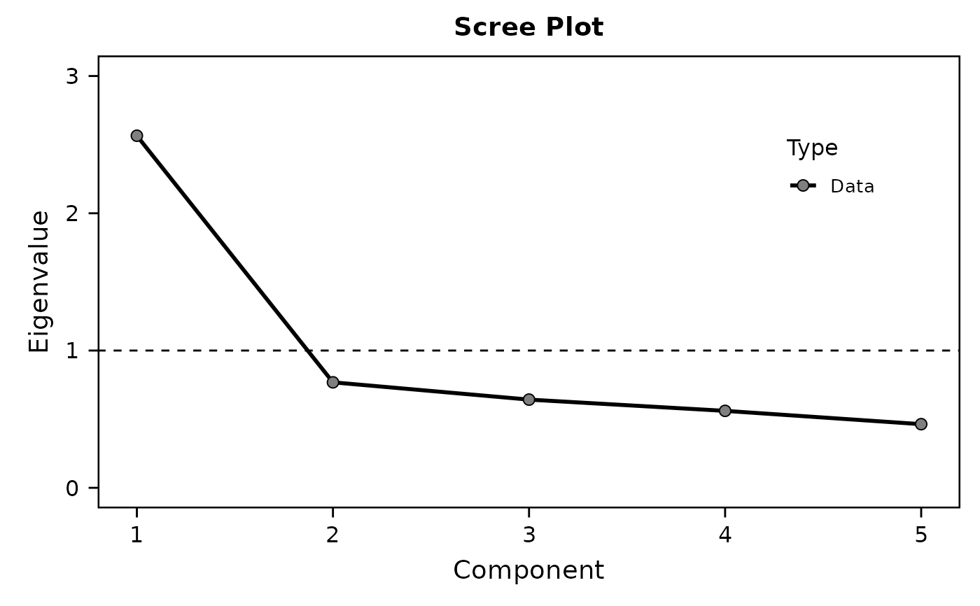
EFA(data, "E", 1:5) # var + items
#>
#> Principal Component Analysis
#>
#> Summary:
#> Total Items: 5
#> Scale Range: 1 ~ 6
#> Total Cases: 2800
#> Valid Cases: 2713 (96.9%)
#>
#> Extraction Method:
#> - Principal Component Analysis
#> Rotation Method:
#> - (Only one component was extracted. The solution was not rotated.)
#>
#> KMO and Bartlett's Test:
#> - Kaiser-Meyer-Olkin (KMO) Measure of Sampling Adequacy: MSA = 0.799
#> - Bartlett's Test of Sphericity: Approx. χ²(10) = 3011.40, p < 1e-99 ***
#>
#> Total Variance Explained:
#> ──────────────────────────────────────────────────────────────────────────────────
#> Eigenvalue Variance % Cumulative % SS Loading Variance % Cumulative %
#> ──────────────────────────────────────────────────────────────────────────────────
#> Component 1 2.565 51.298 51.298 2.565 51.298 51.298
#> Component 2 0.768 15.368 66.666
#> Component 3 0.643 12.851 79.517
#> Component 4 0.561 11.211 90.728
#> Component 5 0.464 9.272 100.000
#> ──────────────────────────────────────────────────────────────────────────────────
#>
#> Component Loadings (Sorted by Size):
#> ──────────────────────
#> PC1 Communality
#> ──────────────────────
#> E2 -0.780 0.608
#> E4 0.758 0.575
#> E1 -0.700 0.490
#> E3 0.691 0.477
#> E5 0.644 0.414
#> ──────────────────────
#> Communality = Sum of Squared (SS) Factor Loadings
#> (Uniqueness = 1 - Communality)
#>
 EFA(data, "E", 1:5, nfactors=2) # var + items
#>
#> Principal Component Analysis
#>
#> Summary:
#> Total Items: 5
#> Scale Range: 1 ~ 6
#> Total Cases: 2800
#> Valid Cases: 2713 (96.9%)
#>
#> Extraction Method:
#> - Principal Component Analysis
#> Rotation Method:
#> - Varimax (with Kaiser Normalization)
#>
#> KMO and Bartlett's Test:
#> - Kaiser-Meyer-Olkin (KMO) Measure of Sampling Adequacy: MSA = 0.799
#> - Bartlett's Test of Sphericity: Approx. χ²(10) = 3011.40, p < 1e-99 ***
#>
#> Total Variance Explained:
#> ──────────────────────────────────────────────────────────────────────────────────
#> Eigenvalue Variance % Cumulative % SS Loading Variance % Cumulative %
#> ──────────────────────────────────────────────────────────────────────────────────
#> Component 1 2.565 51.298 51.298 1.884 37.680 37.680
#> Component 2 0.768 15.368 66.666 1.449 28.986 66.666
#> Component 3 0.643 12.851 79.517
#> Component 4 0.561 11.211 90.728
#> Component 5 0.464 9.272 100.000
#> ──────────────────────────────────────────────────────────────────────────────────
#>
#> Component Loadings (Rotated) (Sorted by Size):
#> ─────────────────────────────
#> RC1 RC2 Communality
#> ─────────────────────────────
#> E1 0.812 -0.098 0.668
#> E2 0.752 -0.304 0.658
#> E4 -0.736 0.290 0.625
#> E5 -0.145 0.860 0.761
#> E3 -0.312 0.723 0.620
#> ─────────────────────────────
#> Communality = Sum of Squared (SS) Factor Loadings
#> (Uniqueness = 1 - Communality)
#>
EFA(data, "E", 1:5, nfactors=2) # var + items
#>
#> Principal Component Analysis
#>
#> Summary:
#> Total Items: 5
#> Scale Range: 1 ~ 6
#> Total Cases: 2800
#> Valid Cases: 2713 (96.9%)
#>
#> Extraction Method:
#> - Principal Component Analysis
#> Rotation Method:
#> - Varimax (with Kaiser Normalization)
#>
#> KMO and Bartlett's Test:
#> - Kaiser-Meyer-Olkin (KMO) Measure of Sampling Adequacy: MSA = 0.799
#> - Bartlett's Test of Sphericity: Approx. χ²(10) = 3011.40, p < 1e-99 ***
#>
#> Total Variance Explained:
#> ──────────────────────────────────────────────────────────────────────────────────
#> Eigenvalue Variance % Cumulative % SS Loading Variance % Cumulative %
#> ──────────────────────────────────────────────────────────────────────────────────
#> Component 1 2.565 51.298 51.298 1.884 37.680 37.680
#> Component 2 0.768 15.368 66.666 1.449 28.986 66.666
#> Component 3 0.643 12.851 79.517
#> Component 4 0.561 11.211 90.728
#> Component 5 0.464 9.272 100.000
#> ──────────────────────────────────────────────────────────────────────────────────
#>
#> Component Loadings (Rotated) (Sorted by Size):
#> ─────────────────────────────
#> RC1 RC2 Communality
#> ─────────────────────────────
#> E1 0.812 -0.098 0.668
#> E2 0.752 -0.304 0.658
#> E4 -0.736 0.290 0.625
#> E5 -0.145 0.860 0.761
#> E3 -0.312 0.723 0.620
#> ─────────────────────────────
#> Communality = Sum of Squared (SS) Factor Loadings
#> (Uniqueness = 1 - Communality)
#>
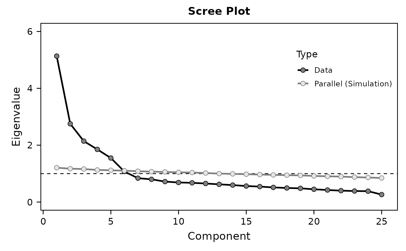
 EFA(data, varrange="A1:O5",
nfactors="parallel",
hide.loadings=0.45)
#>
#> Principal Component Analysis
#>
#> Summary:
#> Total Items: 25
#> Scale Range: 1 ~ 6
#> Total Cases: 2800
#> Valid Cases: 2436 (87.0%)
#>
#> Extraction Method:
#> - Principal Component Analysis
#> Rotation Method:
#> - Varimax (with Kaiser Normalization)
#>
#> KMO and Bartlett's Test:
#> - Kaiser-Meyer-Olkin (KMO) Measure of Sampling Adequacy: MSA = 0.849
#> - Bartlett's Test of Sphericity: Approx. χ²(300) = 18146.07, p < 1e-99 ***
#>
#> Total Variance Explained:
#> ───────────────────────────────────────────────────────────────────────────────────
#> Eigenvalue Variance % Cumulative % SS Loading Variance % Cumulative %
#> ───────────────────────────────────────────────────────────────────────────────────
#> Component 1 5.134 20.537 20.537 3.185 12.738 12.738
#> Component 2 2.752 11.008 31.545 3.100 12.400 25.138
#> Component 3 2.143 8.571 40.116 2.619 10.476 35.615
#> Component 4 1.852 7.409 47.525 2.378 9.512 45.127
#> Component 5 1.548 6.193 53.718 2.148 8.591 53.718
#> Component 6 1.074 4.294 58.012
#> Component 7 0.840 3.358 61.370
#> Component 8 0.799 3.197 64.567
#> Component 9 0.719 2.876 67.443
#> Component 10 0.688 2.752 70.195
#> Component 11 0.676 2.705 72.901
#> Component 12 0.652 2.607 75.508
#> Component 13 0.623 2.493 78.001
#> Component 14 0.597 2.386 80.387
#> Component 15 0.563 2.252 82.640
#> Component 16 0.543 2.173 84.813
#> Component 17 0.515 2.058 86.871
#> Component 18 0.495 1.978 88.849
#> Component 19 0.483 1.931 90.779
#> Component 20 0.449 1.796 92.575
#> Component 21 0.423 1.693 94.269
#> Component 22 0.401 1.603 95.871
#> Component 23 0.388 1.551 97.422
#> Component 24 0.382 1.527 98.950
#> Component 25 0.263 1.050 100.000
#> ───────────────────────────────────────────────────────────────────────────────────
#>
#> Component Loadings (Rotated) (Sorted by Size):
#> ─────────────────────────────────────────────────
#> RC2 RC1 RC3 RC5 RC4 Communality
#> ─────────────────────────────────────────────────
#> N1 0.806 0.710
#> N2 0.794 0.670
#> N3 0.794 0.636
#> N4 0.649 0.587
#> N5 0.631 0.482
#> E2 -0.722 0.608
#> E4 0.700 0.610
#> E1 -0.679 0.478
#> E3 0.625 0.532
#> E5 0.586 0.506
#> C2 0.738 0.579
#> C4 -0.692 0.566
#> C3 0.679 0.478
#> C1 0.654 0.483
#> C5 -0.627 0.532
#> A2 0.716 0.582
#> A3 0.689 0.606
#> A1 -0.638 0.467
#> A5 0.572 0.542
#> A4 0.530 0.424
#> O5 -0.677 0.473
#> O3 0.640 0.561
#> O2 -0.606 0.436
#> O1 0.598 0.444
#> O4 0.494 0.440
#> ─────────────────────────────────────────────────
#> Communality = Sum of Squared (SS) Factor Loadings
#> (Uniqueness = 1 - Communality)
#>
EFA(data, varrange="A1:O5",
nfactors="parallel",
hide.loadings=0.45)
#>
#> Principal Component Analysis
#>
#> Summary:
#> Total Items: 25
#> Scale Range: 1 ~ 6
#> Total Cases: 2800
#> Valid Cases: 2436 (87.0%)
#>
#> Extraction Method:
#> - Principal Component Analysis
#> Rotation Method:
#> - Varimax (with Kaiser Normalization)
#>
#> KMO and Bartlett's Test:
#> - Kaiser-Meyer-Olkin (KMO) Measure of Sampling Adequacy: MSA = 0.849
#> - Bartlett's Test of Sphericity: Approx. χ²(300) = 18146.07, p < 1e-99 ***
#>
#> Total Variance Explained:
#> ───────────────────────────────────────────────────────────────────────────────────
#> Eigenvalue Variance % Cumulative % SS Loading Variance % Cumulative %
#> ───────────────────────────────────────────────────────────────────────────────────
#> Component 1 5.134 20.537 20.537 3.185 12.738 12.738
#> Component 2 2.752 11.008 31.545 3.100 12.400 25.138
#> Component 3 2.143 8.571 40.116 2.619 10.476 35.615
#> Component 4 1.852 7.409 47.525 2.378 9.512 45.127
#> Component 5 1.548 6.193 53.718 2.148 8.591 53.718
#> Component 6 1.074 4.294 58.012
#> Component 7 0.840 3.358 61.370
#> Component 8 0.799 3.197 64.567
#> Component 9 0.719 2.876 67.443
#> Component 10 0.688 2.752 70.195
#> Component 11 0.676 2.705 72.901
#> Component 12 0.652 2.607 75.508
#> Component 13 0.623 2.493 78.001
#> Component 14 0.597 2.386 80.387
#> Component 15 0.563 2.252 82.640
#> Component 16 0.543 2.173 84.813
#> Component 17 0.515 2.058 86.871
#> Component 18 0.495 1.978 88.849
#> Component 19 0.483 1.931 90.779
#> Component 20 0.449 1.796 92.575
#> Component 21 0.423 1.693 94.269
#> Component 22 0.401 1.603 95.871
#> Component 23 0.388 1.551 97.422
#> Component 24 0.382 1.527 98.950
#> Component 25 0.263 1.050 100.000
#> ───────────────────────────────────────────────────────────────────────────────────
#>
#> Component Loadings (Rotated) (Sorted by Size):
#> ─────────────────────────────────────────────────
#> RC2 RC1 RC3 RC5 RC4 Communality
#> ─────────────────────────────────────────────────
#> N1 0.806 0.710
#> N2 0.794 0.670
#> N3 0.794 0.636
#> N4 0.649 0.587
#> N5 0.631 0.482
#> E2 -0.722 0.608
#> E4 0.700 0.610
#> E1 -0.679 0.478
#> E3 0.625 0.532
#> E5 0.586 0.506
#> C2 0.738 0.579
#> C4 -0.692 0.566
#> C3 0.679 0.478
#> C1 0.654 0.483
#> C5 -0.627 0.532
#> A2 0.716 0.582
#> A3 0.689 0.606
#> A1 -0.638 0.467
#> A5 0.572 0.542
#> A4 0.530 0.424
#> O5 -0.677 0.473
#> O3 0.640 0.561
#> O2 -0.606 0.436
#> O1 0.598 0.444
#> O4 0.494 0.440
#> ─────────────────────────────────────────────────
#> Communality = Sum of Squared (SS) Factor Loadings
#> (Uniqueness = 1 - Communality)
#>
 # the same as above:
# using dplyr::select() and dplyr::matches()
# to select variables whose names end with numbers
# (regexp: \d matches all numbers, $ matches the end of a string)
data %>% select(matches("\\d$")) %>%
EFA(vars=names(.), # all selected variables
method="pca", # default
rotation="varimax", # default
nfactors="parallel", # parallel analysis
hide.loadings=0.45) # hide loadings < 0.45
#>
#> Principal Component Analysis
#>
#> Summary:
#> Total Items: 25
#> Scale Range: 1 ~ 6
#> Total Cases: 2800
#> Valid Cases: 2436 (87.0%)
#>
#> Extraction Method:
#> - Principal Component Analysis
#> Rotation Method:
#> - Varimax (with Kaiser Normalization)
#>
#> KMO and Bartlett's Test:
#> - Kaiser-Meyer-Olkin (KMO) Measure of Sampling Adequacy: MSA = 0.849
#> - Bartlett's Test of Sphericity: Approx. χ²(300) = 18146.07, p < 1e-99 ***
#>
#> Total Variance Explained:
#> ───────────────────────────────────────────────────────────────────────────────────
#> Eigenvalue Variance % Cumulative % SS Loading Variance % Cumulative %
#> ───────────────────────────────────────────────────────────────────────────────────
#> Component 1 5.134 20.537 20.537 3.185 12.738 12.738
#> Component 2 2.752 11.008 31.545 3.100 12.400 25.138
#> Component 3 2.143 8.571 40.116 2.619 10.476 35.615
#> Component 4 1.852 7.409 47.525 2.378 9.512 45.127
#> Component 5 1.548 6.193 53.718 2.148 8.591 53.718
#> Component 6 1.074 4.294 58.012
#> Component 7 0.840 3.358 61.370
#> Component 8 0.799 3.197 64.567
#> Component 9 0.719 2.876 67.443
#> Component 10 0.688 2.752 70.195
#> Component 11 0.676 2.705 72.901
#> Component 12 0.652 2.607 75.508
#> Component 13 0.623 2.493 78.001
#> Component 14 0.597 2.386 80.387
#> Component 15 0.563 2.252 82.640
#> Component 16 0.543 2.173 84.813
#> Component 17 0.515 2.058 86.871
#> Component 18 0.495 1.978 88.849
#> Component 19 0.483 1.931 90.779
#> Component 20 0.449 1.796 92.575
#> Component 21 0.423 1.693 94.269
#> Component 22 0.401 1.603 95.871
#> Component 23 0.388 1.551 97.422
#> Component 24 0.382 1.527 98.950
#> Component 25 0.263 1.050 100.000
#> ───────────────────────────────────────────────────────────────────────────────────
#>
#> Component Loadings (Rotated) (Sorted by Size):
#> ─────────────────────────────────────────────────
#> RC2 RC1 RC3 RC5 RC4 Communality
#> ─────────────────────────────────────────────────
#> N1 0.806 0.710
#> N2 0.794 0.670
#> N3 0.794 0.636
#> N4 0.649 0.587
#> N5 0.631 0.482
#> E2 -0.722 0.608
#> E4 0.700 0.610
#> E1 -0.679 0.478
#> E3 0.625 0.532
#> E5 0.586 0.506
#> C2 0.738 0.579
#> C4 -0.692 0.566
#> C3 0.679 0.478
#> C1 0.654 0.483
#> C5 -0.627 0.532
#> A2 0.716 0.582
#> A3 0.689 0.606
#> A1 -0.638 0.467
#> A5 0.572 0.542
#> A4 0.530 0.424
#> O5 -0.677 0.473
#> O3 0.640 0.561
#> O2 -0.606 0.436
#> O1 0.598 0.444
#> O4 0.494 0.440
#> ─────────────────────────────────────────────────
#> Communality = Sum of Squared (SS) Factor Loadings
#> (Uniqueness = 1 - Communality)
#>
# the same as above:
# using dplyr::select() and dplyr::matches()
# to select variables whose names end with numbers
# (regexp: \d matches all numbers, $ matches the end of a string)
data %>% select(matches("\\d$")) %>%
EFA(vars=names(.), # all selected variables
method="pca", # default
rotation="varimax", # default
nfactors="parallel", # parallel analysis
hide.loadings=0.45) # hide loadings < 0.45
#>
#> Principal Component Analysis
#>
#> Summary:
#> Total Items: 25
#> Scale Range: 1 ~ 6
#> Total Cases: 2800
#> Valid Cases: 2436 (87.0%)
#>
#> Extraction Method:
#> - Principal Component Analysis
#> Rotation Method:
#> - Varimax (with Kaiser Normalization)
#>
#> KMO and Bartlett's Test:
#> - Kaiser-Meyer-Olkin (KMO) Measure of Sampling Adequacy: MSA = 0.849
#> - Bartlett's Test of Sphericity: Approx. χ²(300) = 18146.07, p < 1e-99 ***
#>
#> Total Variance Explained:
#> ───────────────────────────────────────────────────────────────────────────────────
#> Eigenvalue Variance % Cumulative % SS Loading Variance % Cumulative %
#> ───────────────────────────────────────────────────────────────────────────────────
#> Component 1 5.134 20.537 20.537 3.185 12.738 12.738
#> Component 2 2.752 11.008 31.545 3.100 12.400 25.138
#> Component 3 2.143 8.571 40.116 2.619 10.476 35.615
#> Component 4 1.852 7.409 47.525 2.378 9.512 45.127
#> Component 5 1.548 6.193 53.718 2.148 8.591 53.718
#> Component 6 1.074 4.294 58.012
#> Component 7 0.840 3.358 61.370
#> Component 8 0.799 3.197 64.567
#> Component 9 0.719 2.876 67.443
#> Component 10 0.688 2.752 70.195
#> Component 11 0.676 2.705 72.901
#> Component 12 0.652 2.607 75.508
#> Component 13 0.623 2.493 78.001
#> Component 14 0.597 2.386 80.387
#> Component 15 0.563 2.252 82.640
#> Component 16 0.543 2.173 84.813
#> Component 17 0.515 2.058 86.871
#> Component 18 0.495 1.978 88.849
#> Component 19 0.483 1.931 90.779
#> Component 20 0.449 1.796 92.575
#> Component 21 0.423 1.693 94.269
#> Component 22 0.401 1.603 95.871
#> Component 23 0.388 1.551 97.422
#> Component 24 0.382 1.527 98.950
#> Component 25 0.263 1.050 100.000
#> ───────────────────────────────────────────────────────────────────────────────────
#>
#> Component Loadings (Rotated) (Sorted by Size):
#> ─────────────────────────────────────────────────
#> RC2 RC1 RC3 RC5 RC4 Communality
#> ─────────────────────────────────────────────────
#> N1 0.806 0.710
#> N2 0.794 0.670
#> N3 0.794 0.636
#> N4 0.649 0.587
#> N5 0.631 0.482
#> E2 -0.722 0.608
#> E4 0.700 0.610
#> E1 -0.679 0.478
#> E3 0.625 0.532
#> E5 0.586 0.506
#> C2 0.738 0.579
#> C4 -0.692 0.566
#> C3 0.679 0.478
#> C1 0.654 0.483
#> C5 -0.627 0.532
#> A2 0.716 0.582
#> A3 0.689 0.606
#> A1 -0.638 0.467
#> A5 0.572 0.542
#> A4 0.530 0.424
#> O5 -0.677 0.473
#> O3 0.640 0.561
#> O2 -0.606 0.436
#> O1 0.598 0.444
#> O4 0.494 0.440
#> ─────────────────────────────────────────────────
#> Communality = Sum of Squared (SS) Factor Loadings
#> (Uniqueness = 1 - Communality)
#>
