Visualize word vectors with dimensionality reduced using t-SNE.

Visualize word vectors with dimensionality reduced using the t-Distributed Stochastic Neighbor Embedding (t-SNE) method (i.e., projecting high-dimensional vectors into a low-dimensional vector space), implemented by Rtsne::Rtsne(). You should specify a random seed if you expect reproducible results.

Usage

plot_wordvec_tSNE(
  x,
  dims = 2,
  perplexity,
  theta = 0.5,
  colors = NULL,
  seed = NULL,
  custom.Rtsne = NULL
)

Arguments

x

Can be:

• a data.table returned by get_wordvec

• a wordvec (data.table) or embed (matrix) loaded by data_wordvec_load

dims

Output dimensionality: 2 (default, the most common choice) or 3.

perplexity

Perplexity parameter, should not be larger than (number of words - 1) / 3. Defaults to floor((length(dt)-1)/3) (where columns of dt are words). See the Rtsne package for details.

theta

Speed/accuracy trade-off (increase for less accuracy), set to 0 for exact t-SNE. Defaults to 0.5.

colors

A character vector specifying (1) the categories of words (for 2-D plot only) or (2) the exact colors of words (for 2-D and 3-D plot). See examples for its usage.

seed

Random seed for reproducible results. Defaults to NULL.

custom.Rtsne

User-defined Rtsne object using the same dt.

Value

2-D: A ggplot object. You may extract the data from this object using $data.

3-D: Nothing but only the data was invisibly returned, because rgl::plot3d() is "called for the side effect of drawing the plot" and thus cannot return any 3-D plot object.

Download

Download pre-trained word vectors data (.RData): https://psychbruce.github.io/WordVector_RData.pdf

References

Hinton, G. E., & Salakhutdinov, R. R. (2006). Reducing the dimensionality of data with neural networks. Science, 313(5786), 504--507.

van der Maaten, L., & Hinton, G. (2008). Visualizing data using t-SNE. Journal of Machine Learning Research, 9, 2579--2605.

See also

plot_wordvec

plot_network

Examples

d = as_embed(demodata, normalize=TRUE)

dt = get_wordvec(d, cc("
  man, woman,
  king, queen,
  China, Beijing,
  Japan, Tokyo"))

## 2-D (default):
plot_wordvec_tSNE(dt, seed=1234)


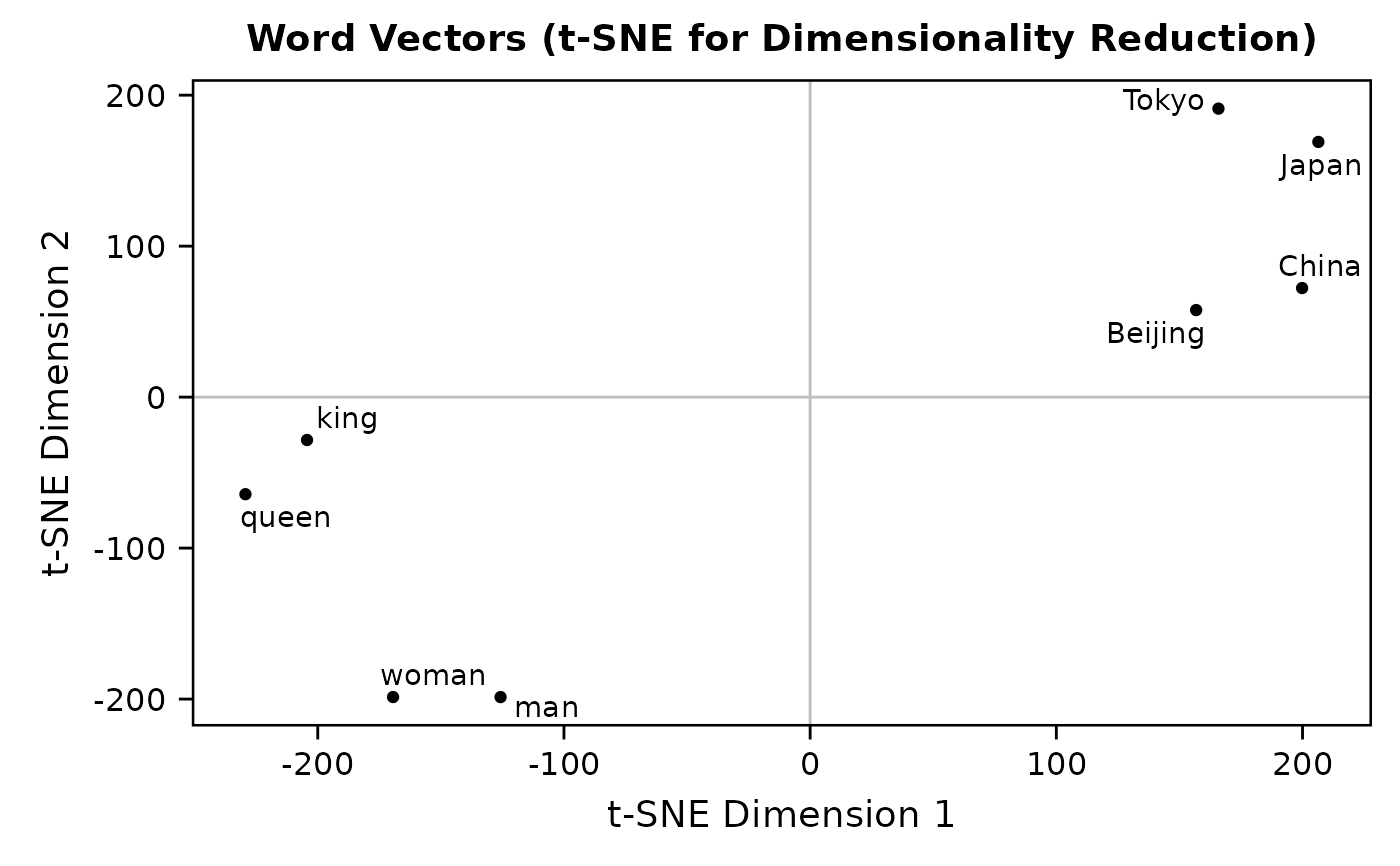plot_wordvec_tSNE(dt, seed=1234)$data
#>      word        V1         V2
#> 1     man -125.7483 -198.68583
#> 2   woman -169.4172 -198.64312
#> 3    king -204.3606  -28.40194
#> 4   queen -229.3772  -64.29560
#> 5   China  199.8315   72.23791
#> 6 Beijing  156.7961   57.66972
#> 7   Japan  206.4292  169.03203
#> 8   Tokyo  165.8464  191.08683

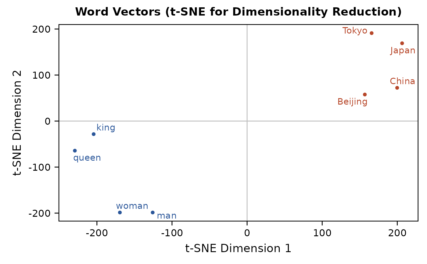
colors = c(rep("#2B579A", 4), rep("#B7472A", 4))
plot_wordvec_tSNE(dt, colors=colors, seed=1234)


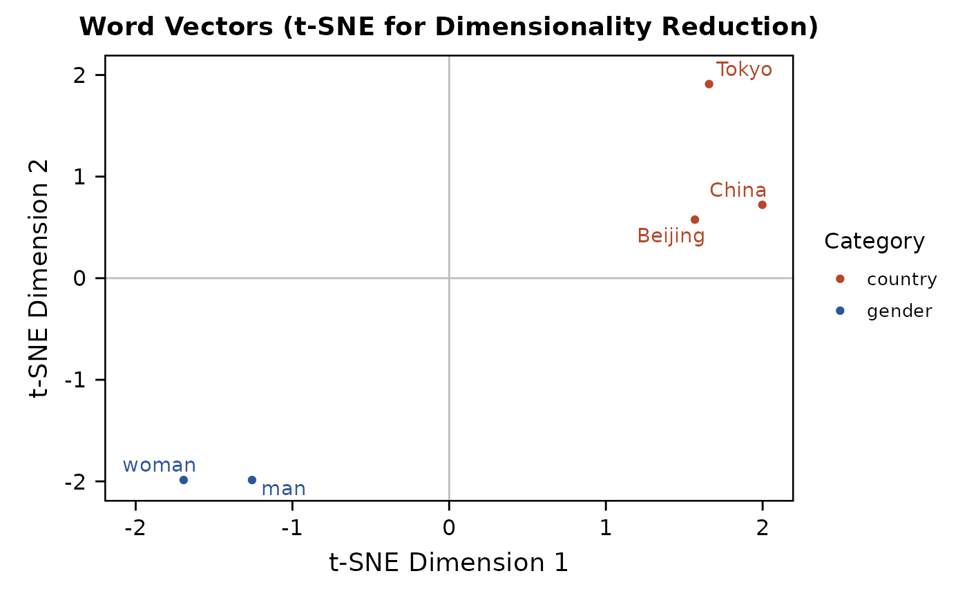
category = c(rep("gender", 4), rep("country", 4))
plot_wordvec_tSNE(dt, colors=category, seed=1234) +
  scale_x_continuous(limits=c(-200, 200),
                     labels=function(x) x/100) +
  scale_y_continuous(limits=c(-200, 200),
                     labels=function(x) x/100) +
  scale_color_manual(values=c("#B7472A", "#2B579A"))
#> Warning: Removed 3 rows containing missing values (`geom_point()`).
#> Warning: Removed 3 rows containing missing values (`geom_text_repel()`).


## 3-D:
colors = c(rep("#2B579A", 4), rep("#B7472A", 4))
plot_wordvec_tSNE(dt, dims=3, colors=colors, seed=1)
#> Warning: RGL: unable to open X11 display
#> Warning: 'rgl.init' failed, running with 'rgl.useNULL = TRUE'.