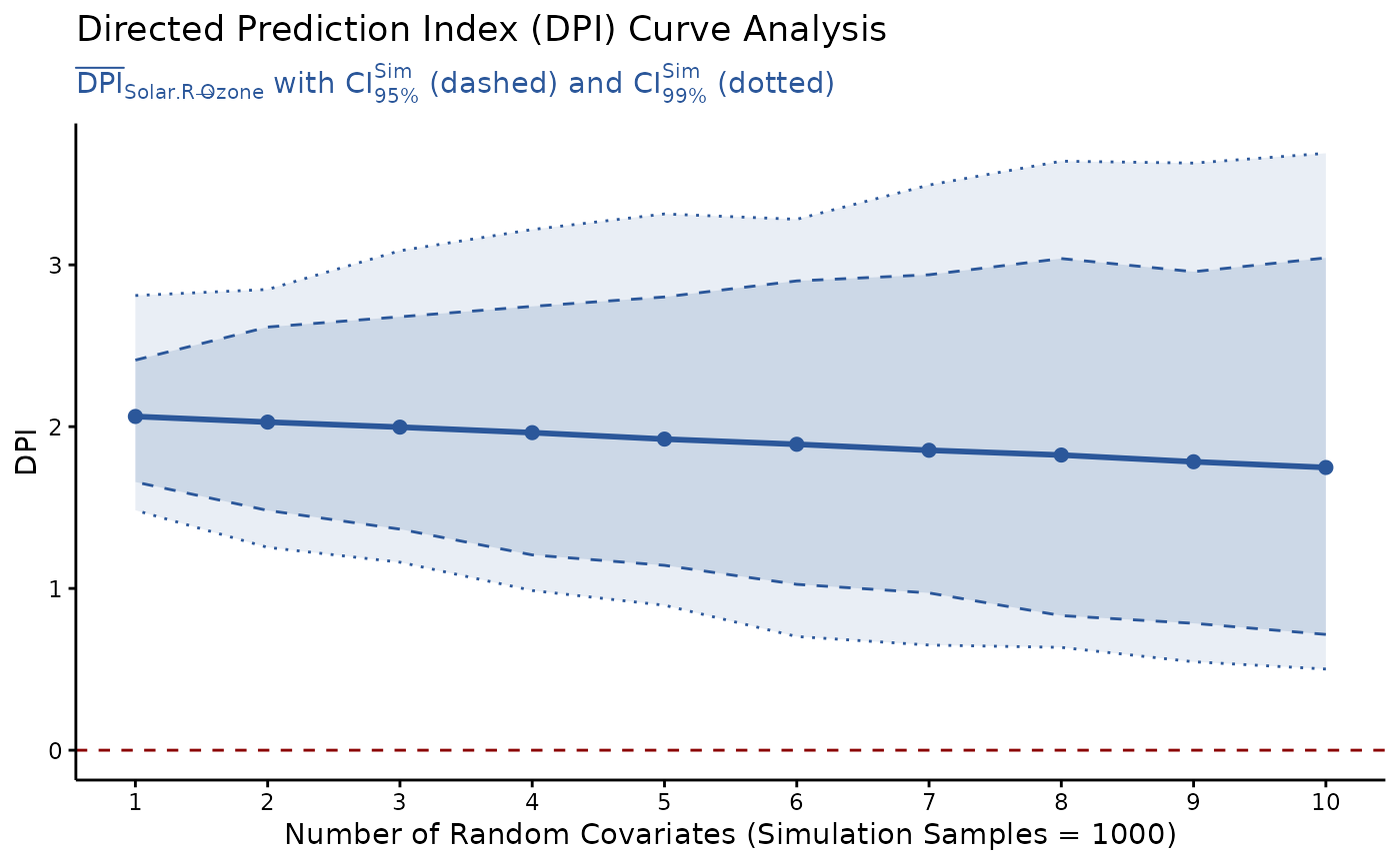
DPI curve analysis across multiple random covariates.

Usage

DPI_curve(
  model,
  x,
  y,
  data = NULL,
  k.covs = 1:10,
  n.sim = 1000,
  alpha = 0.05,
  bonf = FALSE,
  pseudoBF = FALSE,
  seed = NULL,
  progress,
  file = NULL,
  width = 6,
  height = 4,
  dpi = 500
)

Arguments

model

Model object (lm).

x

Independent (predictor) variable.

y

Dependent (outcome) variable.

data

[Optional] Defaults to NULL. If data is specified, then model will be ignored and a linear model lm({y} ~ {x} + .) will be fitted inside. This is helpful for exploring all variables in a dataset.

k.covs

An integer vector of number of random covariates (simulating potential omitted variables) added to each simulation sample. Defaults to 1:10 (producing DPI results for k.cov=1~10). For details, see DPI().

n.sim

Number of simulation samples. Defaults to 1000.

alpha

Significance level for computing the Significance score (0~1) based on p value of partial correlation between X and Y. Defaults to 0.05.

Direction = R2.Y - R2.X
Significance = 1 - tanh(p.beta.xy/alpha/2)

bonf

Bonferroni correction to control for false positive rates: alpha is divided by, and p values are multiplied by, the number of comparisons.

Defaults to FALSE: No correction, suitable if you plan to test only one pair of variables.
TRUE: Using k * (k - 1) / 2 (number of all combinations of variable pairs) where k = length(data).
A user-specified number of comparisons.

pseudoBF

Use normalized pseudo Bayes Factors sigmoid(log(PseudoBF10)) alternatively as the Significance score (0~1). Pseudo Bayes Factors are computed from p value of X-Y partial relationship and total sample size, using the transformation rules proposed by Wagenmakers (2022) doi:10.31234/osf.io/egydq .

Defaults to FALSE because it makes less penalties for insignificant partial relationships between X and Y, see Examples in DPI() and online documentation.

seed

Random seed for replicable results. Defaults to NULL.

progress

Show progress bar. Defaults to TRUE (if length(k.covs) >= 5).

file

File name of saved plot (".png" or ".pdf").

width, height

Width and height (in inches) of saved plot. Defaults to 6 and 4.

dpi

Dots per inch (figure resolution). Defaults to 500.

Value

Return a data.frame of DPI curve results.

Examples

model = lm(Ozone ~ ., data=airquality)
DPIs = DPI_curve(model, x="Solar.R", y="Ozone", seed=1)
#> ⠙ Simulation k.covs: 1/10 ███████████████████████████████   10% [00:00:3.6]
#> ⠹ Simulation k.covs: 2/10 ███████████████████████████████   20% [00:00:7.3]
#> ⠸ Simulation k.covs: 3/10 ███████████████████████████████   30% [00:00:11.5]
#> ⠼ Simulation k.covs: 4/10 ███████████████████████████████   40% [00:00:15.5]
#> ⠴ Simulation k.covs: 5/10 ███████████████████████████████   50% [00:00:19.6]
#> ⠦ Simulation k.covs: 6/10 ███████████████████████████████   60% [00:00:24]
#> ⠧ Simulation k.covs: 7/10 ███████████████████████████████   70% [00:00:28.4]
#> ⠇ Simulation k.covs: 8/10 ███████████████████████████████   80% [00:00:33]
#> ⠏ Simulation k.covs: 9/10 ███████████████████████████████   90% [00:00:37.8]
#> ✔ 10 * 1000 simulation samples estimated in 42.9s
#> 
plot(DPIs)  # ggplot object

DPI curve analysis across multiple random covariates.

Usage

Arguments

Value

See also

Examples