The Directed Prediction Index (DPI) is a causal discovery method for observational data designed to quantify the relative endogeneity of outcome (Y) vs. predictor (X) variables in regression models. By comparing the coefficients of determination (R-squared) between the Y-as-outcome and X-as-outcome models while controlling for sufficient confounders and simulating k random covariates, it can quantify relative endogeneity, providing a necessary but insufficient condition for causal direction from a more exogenous variable (X) to a more endogenous variable (Y). Methodological details are provided at https://psychbruce.github.io/DPI/.
Usage
DPI(
  model,
  x,
  y,
  data = NULL,
  k.cov = 1,
  n.sim = 1000,
  alpha = 0.05,
  bonf = FALSE,
  pseudoBF = FALSE,
  seed = NULL,
  progress,
  file = NULL,
  width = 6,
  height = 4,
  dpi = 500
)
Arguments
- model
Model object (
lm).- x
Independent (predictor) variable.
- y
Dependent (outcome) variable.
- data
[Optional] Defaults to
NULL. Ifdatais specified, thenmodelwill be ignored and a linear modellm({y} ~ {x} + .)will be fitted inside. This is helpful for exploring all variables in a dataset.- k.cov
Number of random covariates (simulating potential omitted variables) added to each simulation sample.
Defaults to
1. Please also test differentk.covvalues as robustness checks (seeDPI_curve()).If
k.cov> 0, the raw data (without bootstrapping) are used, withk.covrandom variables appended, for simulation.If
k.cov= 0 (not suggested), bootstrap samples (resampling with replacement) are used for simulation.
- n.sim
Number of simulation samples. Defaults to
1000.- alpha
Significance level for computing the Normalized Penalty score (0~1) based on p value of partial correlation between
XandY. Defaults to0.05.- bonf
Bonferroni correction to control for false positive rates:
alphais divided by, and p values are multiplied by, the number of comparisons.Defaults to
FALSE: No correction, suitable if you plan to test only one pair of variables.TRUE: Usingk * (k - 1) / 2(all pairs of variables) wherek = length(data).A user-specified number of comparisons.
- pseudoBF
Use normalized pseudo Bayes Factors
sigmoid(log(PseudoBF10))alternatively as the Normalized Penalty score (0~1). Pseudo Bayes Factors are computed from p value of X-Y partial relationship and total sample size, using the transformation rules proposed by Wagenmakers (2022) doi:10.31234/osf.io/egydq .Defaults to
FALSEbecause it makes less penalties for insignificant partial relationships betweenXandY, see Examples inDPI()and online documentation.- seed
Random seed for replicable results. Defaults to
NULL.- progress
Show progress bar. Defaults to
FALSE(ifn.sim< 5000).- file
File name of saved plot (
".png"or".pdf").- width, height
Width and height (in inches) of saved plot. Defaults to
6and4.- dpi
Dots per inch (figure resolution). Defaults to
500.
Value
Return a data.frame of simulation results:
DPI = Relative Endogeneity * Normalized Penalty= (R2.Y - R2.X) * (1 - tanh(p.beta.xy/alpha/2))if
pseudoBF=FALSE(default, suggested)more conservative estimates
= (R2.Y - R2.X) * plogis(log(pseudo.BF.xy))if
pseudoBF=TRUEless conservative for insignificant X-Y relationship
delta.R2R2.Y - R2.X
R2.Y\(R^2\) of regression model predicting Y using X and all other covariates
R2.X\(R^2\) of regression model predicting X using Y and all other covariates
t.beta.xyt value for coefficient of X predicting Y (always equal to t value for coefficient of Y predicting X) when controlling for all other covariates
p.beta.xyp value for coefficient of X predicting Y (always equal to p value for coefficient of Y predicting X) when controlling for all other covariates
df.beta.xyresidual degree of freedom (df) of
t.beta.xy
r.partial.xypartial correlation (always with the same t value as
t.beta.xy) between X and Y when controlling for all other covariates
sigmoid.p.xysigmoid p value as
1 - tanh(p.beta.xy/alpha/2)
pseudo.BF.xypseudo Bayes Factors (\(BF_{10}\)) computed from p value
p.beta.xyand sample sizenobs(model), seep_to_bf()
Examples
# input a fitted model
model = lm(Ozone ~ ., data=airquality)
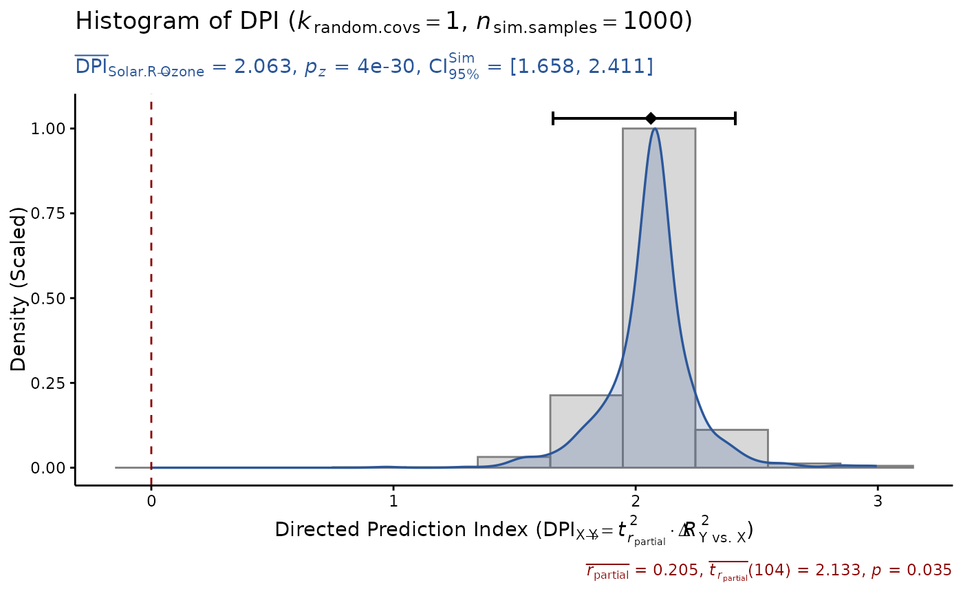
DPI(model, x="Solar.R", y="Ozone", seed=1) # DPI > 0
#> Sample size: N.valid = 111
#> Model Y formula: Ozone ~ Solar.R + Wind + Temp + Month + Day
#> Model X formula: Solar.R ~ Ozone + Wind + Temp + Month + Day
#> Directed prediction: "Solar.R" (X) -> "Ozone" (Y)
#> Partial correlation: r.partial = 0.205, p = 0.0353 * (PseudoBF10 = 0.897)
#> Normalized penalty method: Sigmoid(p/alpha) = 1 - tanh(p.xy/alpha/2)
#> Simulation sample setting: k.random.covs = 1, n.sim = 1000, seed = 1
#> False positive rates (FPR) control: Alpha = 0.05 (Bonferroni correction = 1)
#> Estimate Sim.SE z.value p.z sig Conf.Interval log.PseudoBF10
#> DPI 0.297 (0.031) 9.453 3e-21 *** [0.236, 0.359] 43.710
 DPI(model, x="Wind", y="Ozone", seed=1) # DPI > 0
#> Sample size: N.valid = 111
#> Model Y formula: Ozone ~ Wind + Solar.R + Temp + Month + Day
#> Model X formula: Wind ~ Ozone + Solar.R + Temp + Month + Day
#> Directed prediction: "Wind" (X) -> "Ozone" (Y)
#> Partial correlation: r.partial = -0.449, p = 1e-06 *** (PseudoBF10 = 23117.101)
#> Normalized penalty method: Sigmoid(p/alpha) = 1 - tanh(p.xy/alpha/2)
#> Simulation sample setting: k.random.covs = 1, n.sim = 1000, seed = 1
#> False positive rates (FPR) control: Alpha = 0.05 (Bonferroni correction = 1)
#> Estimate Sim.SE z.value p.z sig Conf.Interval log.PseudoBF10
#> DPI 0.223 (0.009) 25.296 <1e-99 *** [0.206, 0.240] 319.946
DPI(model, x="Wind", y="Ozone", seed=1) # DPI > 0
#> Sample size: N.valid = 111
#> Model Y formula: Ozone ~ Wind + Solar.R + Temp + Month + Day
#> Model X formula: Wind ~ Ozone + Solar.R + Temp + Month + Day
#> Directed prediction: "Wind" (X) -> "Ozone" (Y)
#> Partial correlation: r.partial = -0.449, p = 1e-06 *** (PseudoBF10 = 23117.101)
#> Normalized penalty method: Sigmoid(p/alpha) = 1 - tanh(p.xy/alpha/2)
#> Simulation sample setting: k.random.covs = 1, n.sim = 1000, seed = 1
#> False positive rates (FPR) control: Alpha = 0.05 (Bonferroni correction = 1)
#> Estimate Sim.SE z.value p.z sig Conf.Interval log.PseudoBF10
#> DPI 0.223 (0.009) 25.296 <1e-99 *** [0.206, 0.240] 319.946
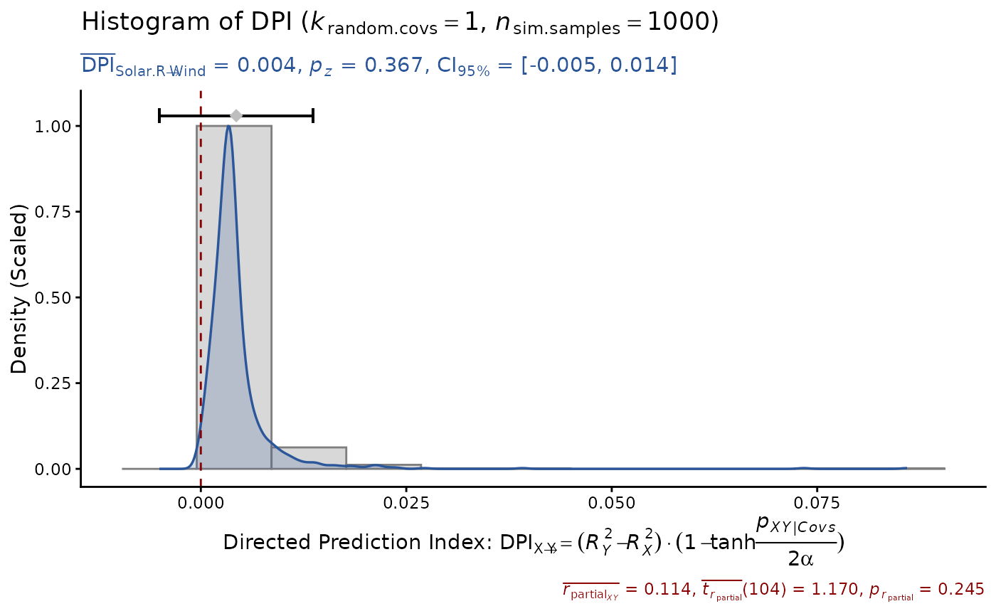
 DPI(model, x="Solar.R", y="Wind", seed=1) # unrelated
#> Sample size: N.valid = 111
#> Model Y formula: Wind ~ Solar.R + Ozone + Temp + Month + Day
#> Model X formula: Solar.R ~ Wind + Ozone + Temp + Month + Day
#> Directed prediction: "Solar.R" (X) -> "Wind" (Y)
#> Partial correlation: r.partial = 0.114, p = 0.2447 (PseudoBF10 = 0.182)
#> Normalized penalty method: Sigmoid(p/alpha) = 1 - tanh(p.xy/alpha/2)
#> Simulation sample setting: k.random.covs = 1, n.sim = 1000, seed = 1
#> False positive rates (FPR) control: Alpha = 0.05 (Bonferroni correction = 1)
#> Estimate Sim.SE z.value p.z sig Conf.Interval log.PseudoBF10
#> DPI 0.004 (0.005) 0.903 0.3666 [-0.005, 0.014] -1.974
DPI(model, x="Solar.R", y="Wind", seed=1) # unrelated
#> Sample size: N.valid = 111
#> Model Y formula: Wind ~ Solar.R + Ozone + Temp + Month + Day
#> Model X formula: Solar.R ~ Wind + Ozone + Temp + Month + Day
#> Directed prediction: "Solar.R" (X) -> "Wind" (Y)
#> Partial correlation: r.partial = 0.114, p = 0.2447 (PseudoBF10 = 0.182)
#> Normalized penalty method: Sigmoid(p/alpha) = 1 - tanh(p.xy/alpha/2)
#> Simulation sample setting: k.random.covs = 1, n.sim = 1000, seed = 1
#> False positive rates (FPR) control: Alpha = 0.05 (Bonferroni correction = 1)
#> Estimate Sim.SE z.value p.z sig Conf.Interval log.PseudoBF10
#> DPI 0.004 (0.005) 0.903 0.3666 [-0.005, 0.014] -1.974
 # or input raw data, test with more random covs
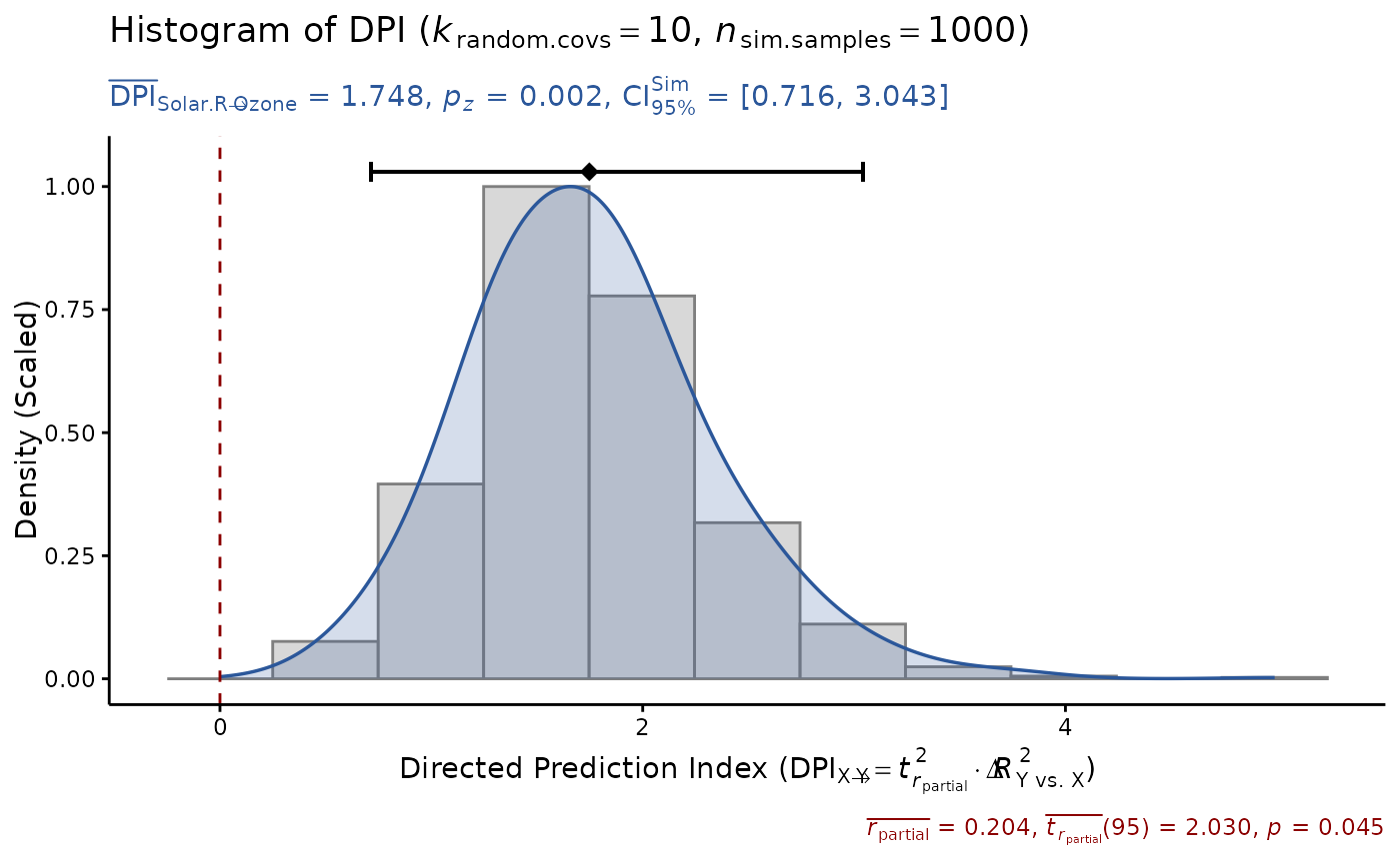
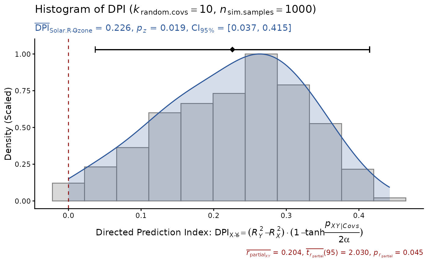
DPI(data=airquality, x="Solar.R", y="Ozone",
k.cov=10, seed=1)
#> Sample size: N.valid = 111
#> Model Y formula: Ozone ~ Solar.R + Wind + Temp + Month + Day
#> Model X formula: Solar.R ~ Ozone + Wind + Temp + Month + Day
#> Directed prediction: "Solar.R" (X) -> "Ozone" (Y)
#> Partial correlation: r.partial = 0.204, p = 0.0452 * (PseudoBF10 = 0.700)
#> Normalized penalty method: Sigmoid(p/alpha) = 1 - tanh(p.xy/alpha/2)
#> Simulation sample setting: k.random.covs = 10, n.sim = 1000, seed = 1
#> False positive rates (FPR) control: Alpha = 0.05 (Bonferroni correction = 1)
#> Estimate Sim.SE z.value p.z sig Conf.Interval log.PseudoBF10
#> DPI 0.226 (0.096) 2.342 0.0192 * [0.037, 0.415] 0.501
# or input raw data, test with more random covs
DPI(data=airquality, x="Solar.R", y="Ozone",
k.cov=10, seed=1)
#> Sample size: N.valid = 111
#> Model Y formula: Ozone ~ Solar.R + Wind + Temp + Month + Day
#> Model X formula: Solar.R ~ Ozone + Wind + Temp + Month + Day
#> Directed prediction: "Solar.R" (X) -> "Ozone" (Y)
#> Partial correlation: r.partial = 0.204, p = 0.0452 * (PseudoBF10 = 0.700)
#> Normalized penalty method: Sigmoid(p/alpha) = 1 - tanh(p.xy/alpha/2)
#> Simulation sample setting: k.random.covs = 10, n.sim = 1000, seed = 1
#> False positive rates (FPR) control: Alpha = 0.05 (Bonferroni correction = 1)
#> Estimate Sim.SE z.value p.z sig Conf.Interval log.PseudoBF10
#> DPI 0.226 (0.096) 2.342 0.0192 * [0.037, 0.415] 0.501
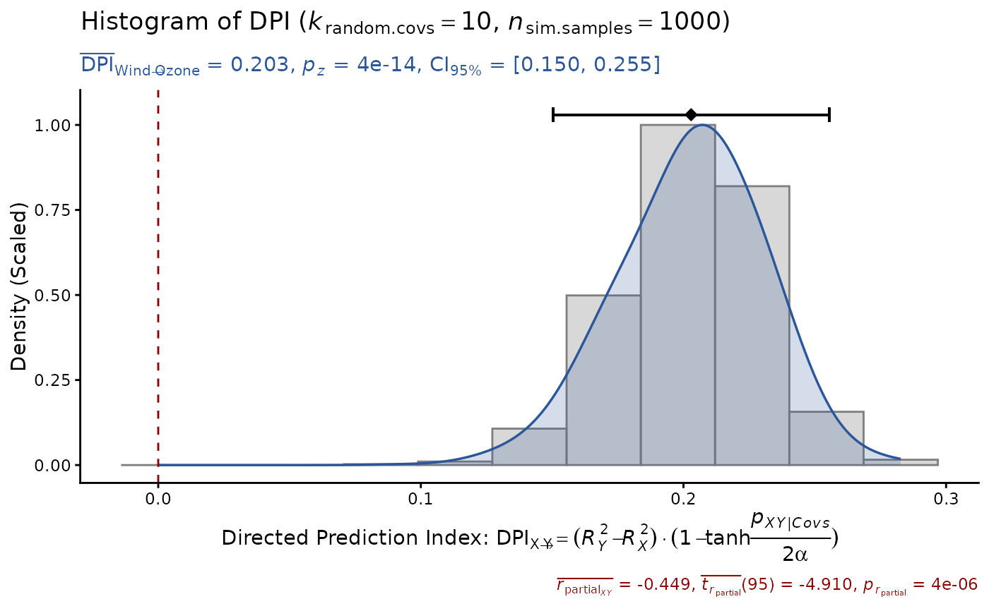
 DPI(data=airquality, x="Wind", y="Ozone",
k.cov=10, seed=1)
#> Sample size: N.valid = 111
#> Model Y formula: Ozone ~ Wind + Solar.R + Temp + Month + Day
#> Model X formula: Wind ~ Ozone + Solar.R + Temp + Month + Day
#> Directed prediction: "Wind" (X) -> "Ozone" (Y)
#> Partial correlation: r.partial = -0.449, p = 4e-06 *** (PseudoBF10 = 8372.103)
#> Normalized penalty method: Sigmoid(p/alpha) = 1 - tanh(p.xy/alpha/2)
#> Simulation sample setting: k.random.covs = 10, n.sim = 1000, seed = 1
#> False positive rates (FPR) control: Alpha = 0.05 (Bonferroni correction = 1)
#> Estimate Sim.SE z.value p.z sig Conf.Interval log.PseudoBF10
#> DPI 0.203 (0.027) 7.567 4e-14 *** [0.150, 0.255] 27.442
DPI(data=airquality, x="Wind", y="Ozone",
k.cov=10, seed=1)
#> Sample size: N.valid = 111
#> Model Y formula: Ozone ~ Wind + Solar.R + Temp + Month + Day
#> Model X formula: Wind ~ Ozone + Solar.R + Temp + Month + Day
#> Directed prediction: "Wind" (X) -> "Ozone" (Y)
#> Partial correlation: r.partial = -0.449, p = 4e-06 *** (PseudoBF10 = 8372.103)
#> Normalized penalty method: Sigmoid(p/alpha) = 1 - tanh(p.xy/alpha/2)
#> Simulation sample setting: k.random.covs = 10, n.sim = 1000, seed = 1
#> False positive rates (FPR) control: Alpha = 0.05 (Bonferroni correction = 1)
#> Estimate Sim.SE z.value p.z sig Conf.Interval log.PseudoBF10
#> DPI 0.203 (0.027) 7.567 4e-14 *** [0.150, 0.255] 27.442
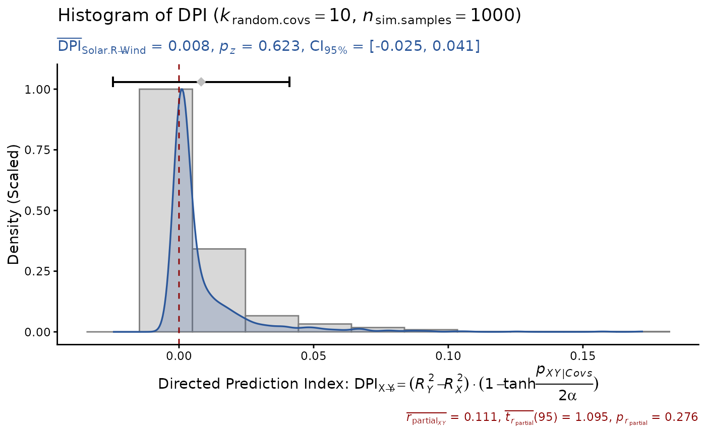
 DPI(data=airquality, x="Solar.R", y="Wind",
k.cov=10, seed=1)
#> Sample size: N.valid = 111
#> Model Y formula: Wind ~ Solar.R + Ozone + Temp + Month + Day
#> Model X formula: Solar.R ~ Wind + Ozone + Temp + Month + Day
#> Directed prediction: "Solar.R" (X) -> "Wind" (Y)
#> Partial correlation: r.partial = 0.111, p = 0.2765 (PseudoBF10 = 0.168)
#> Normalized penalty method: Sigmoid(p/alpha) = 1 - tanh(p.xy/alpha/2)
#> Simulation sample setting: k.random.covs = 10, n.sim = 1000, seed = 1
#> False positive rates (FPR) control: Alpha = 0.05 (Bonferroni correction = 1)
#> Estimate Sim.SE z.value p.z sig Conf.Interval log.PseudoBF10
#> DPI 0.008 (0.017) 0.492 0.6225 [-0.025, 0.041] -2.236
DPI(data=airquality, x="Solar.R", y="Wind",
k.cov=10, seed=1)
#> Sample size: N.valid = 111
#> Model Y formula: Wind ~ Solar.R + Ozone + Temp + Month + Day
#> Model X formula: Solar.R ~ Wind + Ozone + Temp + Month + Day
#> Directed prediction: "Solar.R" (X) -> "Wind" (Y)
#> Partial correlation: r.partial = 0.111, p = 0.2765 (PseudoBF10 = 0.168)
#> Normalized penalty method: Sigmoid(p/alpha) = 1 - tanh(p.xy/alpha/2)
#> Simulation sample setting: k.random.covs = 10, n.sim = 1000, seed = 1
#> False positive rates (FPR) control: Alpha = 0.05 (Bonferroni correction = 1)
#> Estimate Sim.SE z.value p.z sig Conf.Interval log.PseudoBF10
#> DPI 0.008 (0.017) 0.492 0.6225 [-0.025, 0.041] -2.236
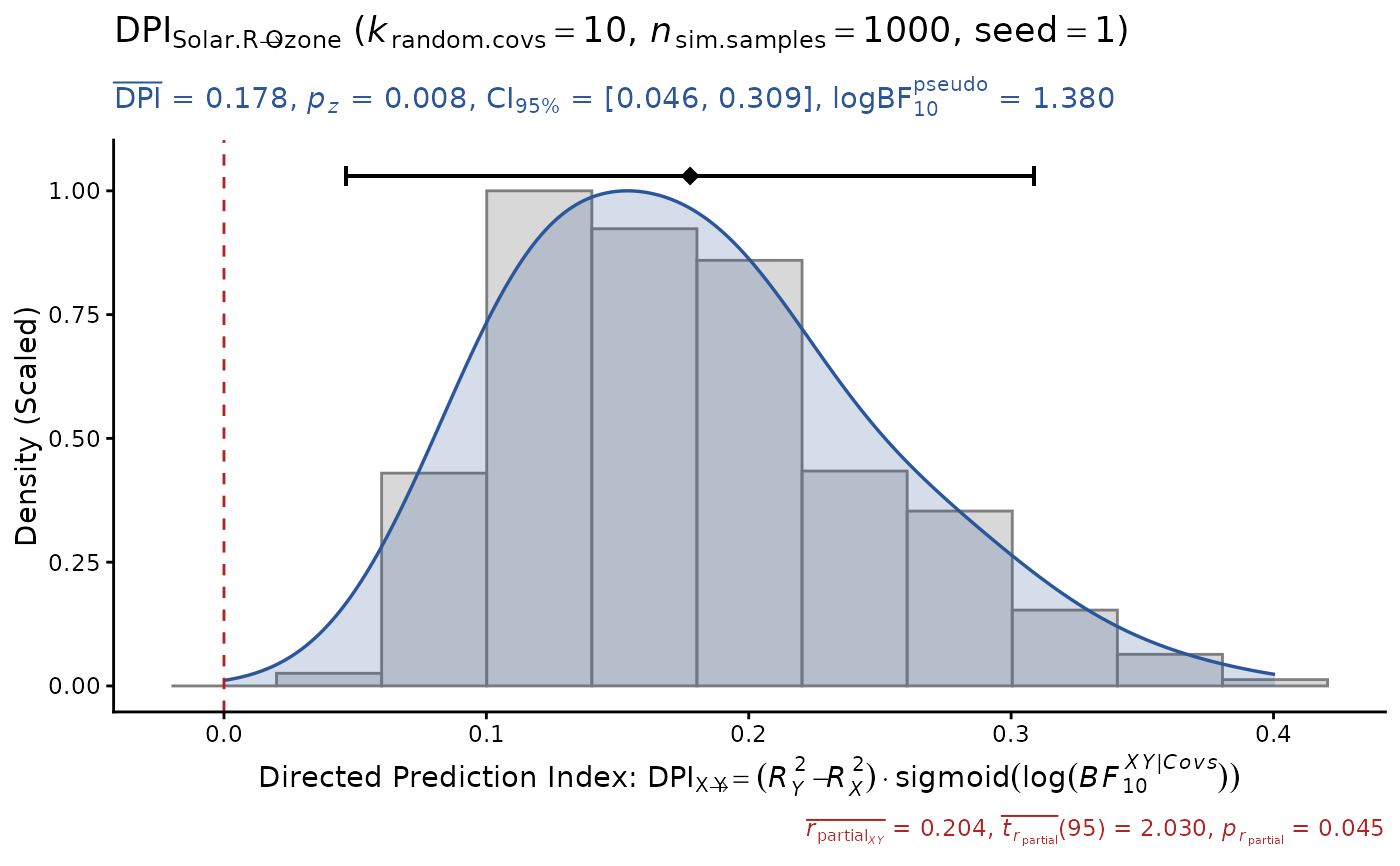
 # or use pseudo Bayes Factors for normalized penalty
# (less conservative for insignificant X-Y relationship)
DPI(data=airquality, x="Solar.R", y="Ozone", k.cov=10,
pseudoBF=TRUE, seed=1) # DPI > 0 (true positive)
#> Sample size: N.valid = 111
#> Model Y formula: Ozone ~ Solar.R + Wind + Temp + Month + Day
#> Model X formula: Solar.R ~ Ozone + Wind + Temp + Month + Day
#> Directed prediction: "Solar.R" (X) -> "Ozone" (Y)
#> Partial correlation: r.partial = 0.204, p = 0.0452 * (PseudoBF10 = 0.700)
#> Normalized penalty method: Sigmoid(log(PseudoBF10.xy))
#> Simulation sample setting: k.random.covs = 10, n.sim = 1000, seed = 1
#> False positive rates (FPR) control: Alpha = 0.05 (Bonferroni correction = 1)
#> Estimate Sim.SE z.value p.z sig Conf.Interval log.PseudoBF10
#> DPI 0.178 (0.067) 2.654 0.0080 ** [0.046, 0.309] 1.380
# or use pseudo Bayes Factors for normalized penalty
# (less conservative for insignificant X-Y relationship)
DPI(data=airquality, x="Solar.R", y="Ozone", k.cov=10,
pseudoBF=TRUE, seed=1) # DPI > 0 (true positive)
#> Sample size: N.valid = 111
#> Model Y formula: Ozone ~ Solar.R + Wind + Temp + Month + Day
#> Model X formula: Solar.R ~ Ozone + Wind + Temp + Month + Day
#> Directed prediction: "Solar.R" (X) -> "Ozone" (Y)
#> Partial correlation: r.partial = 0.204, p = 0.0452 * (PseudoBF10 = 0.700)
#> Normalized penalty method: Sigmoid(log(PseudoBF10.xy))
#> Simulation sample setting: k.random.covs = 10, n.sim = 1000, seed = 1
#> False positive rates (FPR) control: Alpha = 0.05 (Bonferroni correction = 1)
#> Estimate Sim.SE z.value p.z sig Conf.Interval log.PseudoBF10
#> DPI 0.178 (0.067) 2.654 0.0080 ** [0.046, 0.309] 1.380
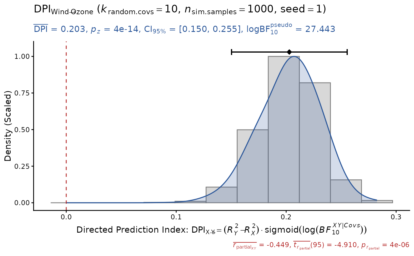
 DPI(data=airquality, x="Wind", y="Ozone", k.cov=10,
pseudoBF=TRUE, seed=1) # DPI > 0 (true positive)
#> Sample size: N.valid = 111
#> Model Y formula: Ozone ~ Wind + Solar.R + Temp + Month + Day
#> Model X formula: Wind ~ Ozone + Solar.R + Temp + Month + Day
#> Directed prediction: "Wind" (X) -> "Ozone" (Y)
#> Partial correlation: r.partial = -0.449, p = 4e-06 *** (PseudoBF10 = 8372.103)
#> Normalized penalty method: Sigmoid(log(PseudoBF10.xy))
#> Simulation sample setting: k.random.covs = 10, n.sim = 1000, seed = 1
#> False positive rates (FPR) control: Alpha = 0.05 (Bonferroni correction = 1)
#> Estimate Sim.SE z.value p.z sig Conf.Interval log.PseudoBF10
#> DPI 0.203 (0.027) 7.567 4e-14 *** [0.150, 0.255] 27.443
DPI(data=airquality, x="Wind", y="Ozone", k.cov=10,
pseudoBF=TRUE, seed=1) # DPI > 0 (true positive)
#> Sample size: N.valid = 111
#> Model Y formula: Ozone ~ Wind + Solar.R + Temp + Month + Day
#> Model X formula: Wind ~ Ozone + Solar.R + Temp + Month + Day
#> Directed prediction: "Wind" (X) -> "Ozone" (Y)
#> Partial correlation: r.partial = -0.449, p = 4e-06 *** (PseudoBF10 = 8372.103)
#> Normalized penalty method: Sigmoid(log(PseudoBF10.xy))
#> Simulation sample setting: k.random.covs = 10, n.sim = 1000, seed = 1
#> False positive rates (FPR) control: Alpha = 0.05 (Bonferroni correction = 1)
#> Estimate Sim.SE z.value p.z sig Conf.Interval log.PseudoBF10
#> DPI 0.203 (0.027) 7.567 4e-14 *** [0.150, 0.255] 27.443
 DPI(data=airquality, x="Solar.R", y="Wind", k.cov=10,
pseudoBF=TRUE, seed=1) # DPI > 0 (false positive!)
#> Sample size: N.valid = 111
#> Model Y formula: Wind ~ Solar.R + Ozone + Temp + Month + Day
#> Model X formula: Solar.R ~ Wind + Ozone + Temp + Month + Day
#> Directed prediction: "Solar.R" (X) -> "Wind" (Y)
#> Partial correlation: r.partial = 0.111, p = 0.2765 (PseudoBF10 = 0.168)
#> Normalized penalty method: Sigmoid(log(PseudoBF10.xy))
#> Simulation sample setting: k.random.covs = 10, n.sim = 1000, seed = 1
#> False positive rates (FPR) control: Alpha = 0.05 (Bonferroni correction = 1)
#> Estimate Sim.SE z.value p.z sig Conf.Interval log.PseudoBF10
#> DPI 0.032 (0.012) 2.767 0.0057 ** [0.009, 0.055] 1.722
DPI(data=airquality, x="Solar.R", y="Wind", k.cov=10,
pseudoBF=TRUE, seed=1) # DPI > 0 (false positive!)
#> Sample size: N.valid = 111
#> Model Y formula: Wind ~ Solar.R + Ozone + Temp + Month + Day
#> Model X formula: Solar.R ~ Wind + Ozone + Temp + Month + Day
#> Directed prediction: "Solar.R" (X) -> "Wind" (Y)
#> Partial correlation: r.partial = 0.111, p = 0.2765 (PseudoBF10 = 0.168)
#> Normalized penalty method: Sigmoid(log(PseudoBF10.xy))
#> Simulation sample setting: k.random.covs = 10, n.sim = 1000, seed = 1
#> False positive rates (FPR) control: Alpha = 0.05 (Bonferroni correction = 1)
#> Estimate Sim.SE z.value p.z sig Conf.Interval log.PseudoBF10
#> DPI 0.032 (0.012) 2.767 0.0057 ** [0.009, 0.055] 1.722
